Post History
For any 2nd order low pass filter, the components (R, L and C for electrical and k, M and c for mechanical) can be reduced into two more meaningful quantities: - $\zeta$ (the damping ratio) $\omeg...
#6: Post edited
by
 Andy aka
·
2020-06-20T11:07:00Z (almost 5 years ago)
Andy aka
·
2020-06-20T11:07:00Z (almost 5 years ago)
For any 2nd order low pass filter be it electrical or mechanical, the components (R, L and C for [electrical](https://en.wikipedia.org/wiki/RLC_circuit#Series_circuit) and k, M and c for [mechanical](https://en.wikipedia.org/wiki/Damping_ratio#Definition)) can be broken down into two quantities: -- - \$\zeta\$ (the damping ratio)
- - \$\omega_n\$ (the natural resonant frequency)
Concentrating on the RLC circuit in the question: -- - \$\zeta = \dfrac{R}{2}\sqrt{\dfrac{C}{L}}\$ and,
- - \$\omega_n = \dfrac{1}{\sqrt{LC}}\$
- # Bode plot
A typical 2nd order low pass filter amplitude response bode plot: -- 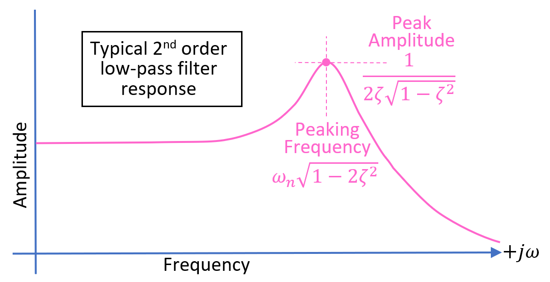
- # 3-D picture introducing pole-zero diagram
Here's the bigger picture of the bode plot when combined with the pole zero diagram (only the positive pole is shown for clarity reasons): -- 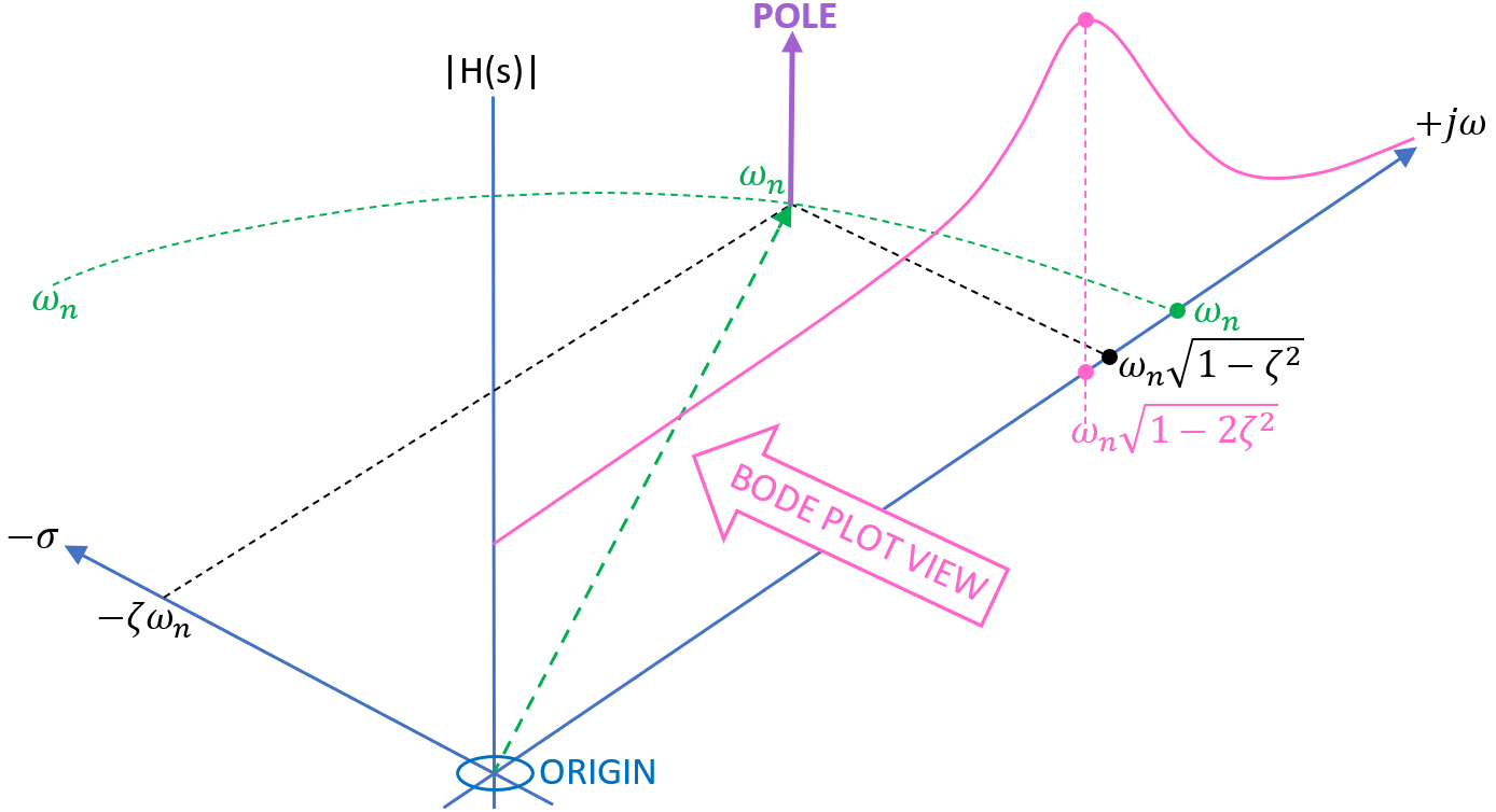
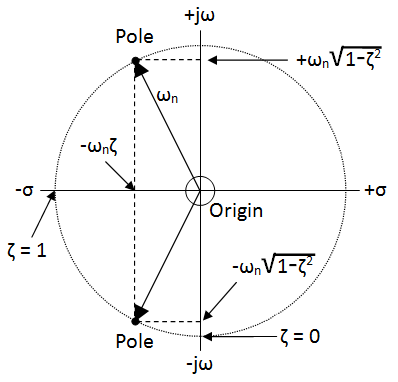
- # Traditional pole zero diagram
- Looking down onto the above 3-D picture shows the traditional pole zero diagram (both poles shown): -
- 
- # Pole zero geometry and |H(s)|
- If you know the pole positions (or the zero positions) you can predict the bode plot magnitude by calculating the distance from each pole (or zero) to any particular point on the bode plot. This reveals the magnitude along the jω axis. Note that the red dot below is a variable point on the jω axis that is required to be calculated. The geometry of the pole zero diagram is examined: -
- 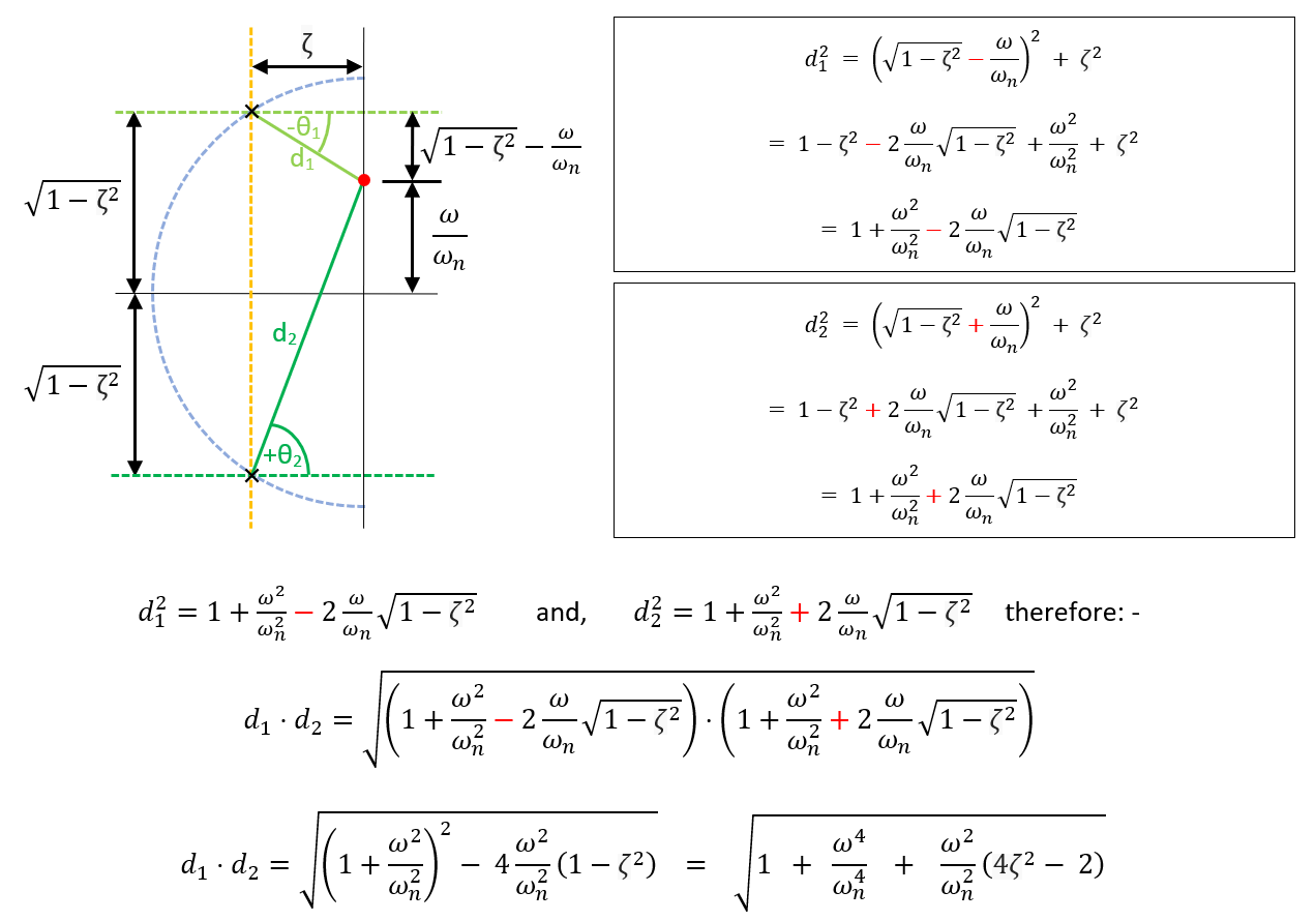
- The reciprocal of d1⋅d2 gives you the magnitude of the bode plot at any point on the jω axis. If there was a zero involved (at a distance n1 to the particular point on the jω axis), the magnitude would be the reciprocal of: -
- $$\dfrac{d_1⋅d_2}{n_1}$$
- Some pictures from [here](http://stades.co.uk/index.html).
- # Pole zero diagram and phase response
- The phase response is derived from the pole zero diagram. Here it is using the conjugate pole example from above: -
- 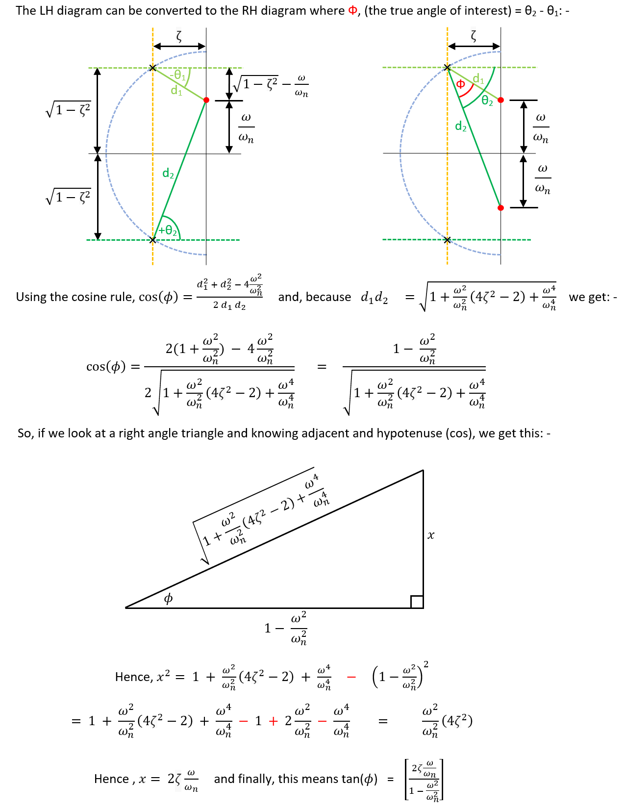
- But, of course, you could just take the transfer function and mathematically derive phase and magnitude response without reference to the geometry of the pole zero diagram.
- For any 2nd order low pass filter, the components (R, L and C for [electrical](https://en.wikipedia.org/wiki/RLC_circuit#Series_circuit) and k, M and c for [mechanical](https://en.wikipedia.org/wiki/Damping_ratio#Definition)) can be reduced into two more meaningful quantities: -
- - \$\zeta\$ (the damping ratio)
- - \$\omega_n\$ (the natural resonant frequency)
- Concentrating on the RLC circuit in the question, these relationships hold: -
- - \$\zeta = \dfrac{R}{2}\sqrt{\dfrac{C}{L}}\$ and,
- - \$\omega_n = \dfrac{1}{\sqrt{LC}}\$
- # Bode plot
- The amplitude section of the bode plot will be similar to this: -
- 
- # 3-D picture introducing pole-zero diagram
- The bode plot and pole zero diagram are combined. Only the positive pole is shown for clarity: -
- 
- # Traditional pole zero diagram
- Looking down onto the above 3-D picture shows the traditional pole zero diagram (both poles shown): -
- 
- # Pole zero geometry and |H(s)|
- If you know the pole positions (or the zero positions) you can predict the bode plot magnitude by calculating the distance from each pole (or zero) to any particular point on the bode plot. This reveals the magnitude along the jω axis. Note that the red dot below is a variable point on the jω axis that is required to be calculated. The geometry of the pole zero diagram is examined: -
- 
- The reciprocal of d1⋅d2 gives you the magnitude of the bode plot at any point on the jω axis. If there was a zero involved (at a distance n1 to the particular point on the jω axis), the magnitude would be the reciprocal of: -
- $$\dfrac{d_1⋅d_2}{n_1}$$
- Some pictures from [here](http://stades.co.uk/index.html).
- # Pole zero diagram and phase response
- The phase response is derived from the pole zero diagram. Here it is using the conjugate pole example from above: -
- 
- But, of course, you could just take the transfer function and mathematically derive phase and magnitude response without reference to the geometry of the pole zero diagram.
#5: Post edited
by
Andy aka
·
2020-06-19T12:17:24Z (about 5 years ago)
For any 2nd order low pass filter be it electrical or mechanical, the components (R, L and C for electrical and k, M and c for mechanical) can be broken down into two quantities: -- - \$\zeta\$ (the damping ratio)
- - \$\omega_n\$ (the natural resonant frequency)
For the RLC circuit in the question, \$\zeta = \dfrac{R}{2}\sqrt{\dfrac{C}{L}}\$ and \$\omega_n = \dfrac{1}{\sqrt{LC}}\$- # Bode plot
- A typical 2nd order low pass filter amplitude response bode plot: -
- 
- # 3-D picture introducing pole-zero diagram
- Here's the bigger picture of the bode plot when combined with the pole zero diagram (only the positive pole is shown for clarity reasons): -
- 
- # Traditional pole zero diagram
- Looking down onto the above 3-D picture shows the traditional pole zero diagram (both poles shown): -
- 
- # Pole zero geometry and |H(s)|
- If you know the pole positions (or the zero positions) you can predict the bode plot magnitude by calculating the distance from each pole (or zero) to any particular point on the bode plot. This reveals the magnitude along the jω axis. Note that the red dot below is a variable point on the jω axis that is required to be calculated. The geometry of the pole zero diagram is examined: -
- 
- The reciprocal of d1⋅d2 gives you the magnitude of the bode plot at any point on the jω axis. If there was a zero involved (at a distance n1 to the particular point on the jω axis), the magnitude would be the reciprocal of: -
- $$\dfrac{d_1⋅d_2}{n_1}$$
- Some pictures from [here](http://stades.co.uk/index.html).
- # Pole zero diagram and phase response
- The phase response is derived from the pole zero diagram. Here it is using the conjugate pole example from above: -
- 
- But, of course, you could just take the transfer function and mathematically derive phase and magnitude response without reference to the geometry of the pole zero diagram.
- For any 2nd order low pass filter be it electrical or mechanical, the components (R, L and C for [electrical](https://en.wikipedia.org/wiki/RLC_circuit#Series_circuit) and k, M and c for [mechanical](https://en.wikipedia.org/wiki/Damping_ratio#Definition)) can be broken down into two quantities: -
- - \$\zeta\$ (the damping ratio)
- - \$\omega_n\$ (the natural resonant frequency)
- Concentrating on the RLC circuit in the question: -
- - \$\zeta = \dfrac{R}{2}\sqrt{\dfrac{C}{L}}\$ and,
- - \$\omega_n = \dfrac{1}{\sqrt{LC}}\$
- # Bode plot
- A typical 2nd order low pass filter amplitude response bode plot: -
- 
- # 3-D picture introducing pole-zero diagram
- Here's the bigger picture of the bode plot when combined with the pole zero diagram (only the positive pole is shown for clarity reasons): -
- 
- # Traditional pole zero diagram
- Looking down onto the above 3-D picture shows the traditional pole zero diagram (both poles shown): -
- 
- # Pole zero geometry and |H(s)|
- If you know the pole positions (or the zero positions) you can predict the bode plot magnitude by calculating the distance from each pole (or zero) to any particular point on the bode plot. This reveals the magnitude along the jω axis. Note that the red dot below is a variable point on the jω axis that is required to be calculated. The geometry of the pole zero diagram is examined: -
- 
- The reciprocal of d1⋅d2 gives you the magnitude of the bode plot at any point on the jω axis. If there was a zero involved (at a distance n1 to the particular point on the jω axis), the magnitude would be the reciprocal of: -
- $$\dfrac{d_1⋅d_2}{n_1}$$
- Some pictures from [here](http://stades.co.uk/index.html).
- # Pole zero diagram and phase response
- The phase response is derived from the pole zero diagram. Here it is using the conjugate pole example from above: -
- 
- But, of course, you could just take the transfer function and mathematically derive phase and magnitude response without reference to the geometry of the pole zero diagram.
#4: Post edited
by
Andy aka
·
2020-06-19T12:09:41Z (about 5 years ago)
- For any 2nd order low pass filter be it electrical or mechanical, the components (R, L and C for electrical and k, M and c for mechanical) can be broken down into two quantities: -
- - \$\zeta\$ (the damping ratio)
- - \$\omega_n\$ (the natural resonant frequency)
- For the RLC circuit in the question, \$\zeta = \dfrac{R}{2}\sqrt{\dfrac{C}{L}}\$ and \$\omega_n = \dfrac{1}{\sqrt{LC}}\$
- # Bode plot
- A typical 2nd order low pass filter amplitude response bode plot: -
- 
- # 3-D picture introducing pole-zero diagram
Here's the bigger picture of the bode plot when combined with the pole zero diagram: -- 
- # Traditional pole zero diagram
Looking down onto the above 3-D picture shows the traditional pole zero diagram: -- 
- # Pole zero geometry and |H(s)|
- If you know the pole positions (or the zero positions) you can predict the bode plot magnitude by calculating the distance from each pole (or zero) to any particular point on the bode plot. This reveals the magnitude along the jω axis. Note that the red dot below is a variable point on the jω axis that is required to be calculated. The geometry of the pole zero diagram is examined: -
- 
- The reciprocal of d1⋅d2 gives you the magnitude of the bode plot at any point on the jω axis. If there was a zero involved (at a distance n1 to the particular point on the jω axis), the magnitude would be the reciprocal of: -
- $$\dfrac{d_1⋅d_2}{n_1}$$
- Some pictures from [here](http://stades.co.uk/index.html).
- # Pole zero diagram and phase response
If you want to know how the phase response is derived from the pole zero diagram, here it is for the conjugate pole example from above: -- 
- But, of course, you could just take the transfer function and mathematically derive phase and magnitude response without reference to the geometry of the pole zero diagram.
- For any 2nd order low pass filter be it electrical or mechanical, the components (R, L and C for electrical and k, M and c for mechanical) can be broken down into two quantities: -
- - \$\zeta\$ (the damping ratio)
- - \$\omega_n\$ (the natural resonant frequency)
- For the RLC circuit in the question, \$\zeta = \dfrac{R}{2}\sqrt{\dfrac{C}{L}}\$ and \$\omega_n = \dfrac{1}{\sqrt{LC}}\$
- # Bode plot
- A typical 2nd order low pass filter amplitude response bode plot: -
- 
- # 3-D picture introducing pole-zero diagram
- Here's the bigger picture of the bode plot when combined with the pole zero diagram (only the positive pole is shown for clarity reasons): -
- 
- # Traditional pole zero diagram
- Looking down onto the above 3-D picture shows the traditional pole zero diagram (both poles shown): -
- 
- # Pole zero geometry and |H(s)|
- If you know the pole positions (or the zero positions) you can predict the bode plot magnitude by calculating the distance from each pole (or zero) to any particular point on the bode plot. This reveals the magnitude along the jω axis. Note that the red dot below is a variable point on the jω axis that is required to be calculated. The geometry of the pole zero diagram is examined: -
- 
- The reciprocal of d1⋅d2 gives you the magnitude of the bode plot at any point on the jω axis. If there was a zero involved (at a distance n1 to the particular point on the jω axis), the magnitude would be the reciprocal of: -
- $$\dfrac{d_1⋅d_2}{n_1}$$
- Some pictures from [here](http://stades.co.uk/index.html).
- # Pole zero diagram and phase response
- The phase response is derived from the pole zero diagram. Here it is using the conjugate pole example from above: -
- 
- But, of course, you could just take the transfer function and mathematically derive phase and magnitude response without reference to the geometry of the pole zero diagram.
#3: Post edited
by
Andy aka
·
2020-06-19T12:04:04Z (about 5 years ago)
- For any 2nd order low pass filter be it electrical or mechanical, the components (R, L and C for electrical and k, M and c for mechanical) can be broken down into two quantities: -
- - \$\zeta\$ (the damping ratio)
- - \$\omega_n\$ (the natural resonant frequency)
- # Bode plot
- A typical 2nd order low pass filter amplitude response bode plot: -
- 
- # 3-D picture introducing pole-zero diagram
- Here's the bigger picture of the bode plot when combined with the pole zero diagram: -
- 
- # Traditional pole zero diagram
- Looking down onto the above 3-D picture shows the traditional pole zero diagram: -
- 
- # Pole zero geometry and |H(s)|
- If you know the pole positions (or the zero positions) you can predict the bode plot magnitude by calculating the distance from each pole (or zero) to any particular point on the bode plot. This reveals the magnitude along the jω axis. Note that the red dot below is a variable point on the jω axis that is required to be calculated. The geometry of the pole zero diagram is examined: -
- 
- The reciprocal of d1⋅d2 gives you the magnitude of the bode plot at any point on the jω axis. If there was a zero involved (at a distance n1 to the particular point on the jω axis), the magnitude would be the reciprocal of: -
- $$\dfrac{d_1⋅d_2}{n_1}$$
- Some pictures from [here](http://stades.co.uk/index.html).
- # Pole zero diagram and phase response
- If you want to know how the phase response is derived from the pole zero diagram, here it is for the conjugate pole example from above: -
- 
- But, of course, you could just take the transfer function and mathematically derive phase and magnitude response without reference to the geometry of the pole zero diagram.
- For any 2nd order low pass filter be it electrical or mechanical, the components (R, L and C for electrical and k, M and c for mechanical) can be broken down into two quantities: -
- - \$\zeta\$ (the damping ratio)
- - \$\omega_n\$ (the natural resonant frequency)
- For the RLC circuit in the question, \$\zeta = \dfrac{R}{2}\sqrt{\dfrac{C}{L}}\$ and \$\omega_n = \dfrac{1}{\sqrt{LC}}\$
- # Bode plot
- A typical 2nd order low pass filter amplitude response bode plot: -
- 
- # 3-D picture introducing pole-zero diagram
- Here's the bigger picture of the bode plot when combined with the pole zero diagram: -
- 
- # Traditional pole zero diagram
- Looking down onto the above 3-D picture shows the traditional pole zero diagram: -
- 
- # Pole zero geometry and |H(s)|
- If you know the pole positions (or the zero positions) you can predict the bode plot magnitude by calculating the distance from each pole (or zero) to any particular point on the bode plot. This reveals the magnitude along the jω axis. Note that the red dot below is a variable point on the jω axis that is required to be calculated. The geometry of the pole zero diagram is examined: -
- 
- The reciprocal of d1⋅d2 gives you the magnitude of the bode plot at any point on the jω axis. If there was a zero involved (at a distance n1 to the particular point on the jω axis), the magnitude would be the reciprocal of: -
- $$\dfrac{d_1⋅d_2}{n_1}$$
- Some pictures from [here](http://stades.co.uk/index.html).
- # Pole zero diagram and phase response
- If you want to know how the phase response is derived from the pole zero diagram, here it is for the conjugate pole example from above: -
- 
- But, of course, you could just take the transfer function and mathematically derive phase and magnitude response without reference to the geometry of the pole zero diagram.
#2: Post edited
by
Andy aka
·
2020-06-19T11:22:12Z (about 5 years ago)
- # Bode plot
Take a typical 2nd order low pass filter amplitude response bode plot: -- 
- # 3-D picture introducing pole-zero diagram
- Here's the bigger picture of the bode plot when combined with the pole zero diagram: -
- 
- # Traditional pole zero diagram
- Looking down onto the above 3-D picture shows the traditional pole zero diagram: -
- 
- # Pole zero geometry and |H(s)|
- If you know the pole positions (or the zero positions) you can predict the bode plot magnitude by calculating the distance from each pole (or zero) to any particular point on the bode plot. This reveals the magnitude along the jω axis. Note that the red dot below is a variable point on the jω axis that is required to be calculated. The geometry of the pole zero diagram is examined: -
- 
- The reciprocal of d1⋅d2 gives you the magnitude of the bode plot at any point on the jω axis. If there was a zero involved (at a distance n1 to the particular point on the jω axis), the magnitude would be the reciprocal of: -
- $$\dfrac{d_1⋅d_2}{n_1}$$
- Some pictures from [here](http://stades.co.uk/index.html).
- # Pole zero diagram and phase response
- If you want to know how the phase response is derived from the pole zero diagram, here it is for the conjugate pole example from above: -
- 
- But, of course, you could just take the transfer function and mathematically derive phase and magnitude response without reference to the geometry of the pole zero diagram.
- For any 2nd order low pass filter be it electrical or mechanical, the components (R, L and C for electrical and k, M and c for mechanical) can be broken down into two quantities: -
- - \$\zeta\$ (the damping ratio)
- - \$\omega_n\$ (the natural resonant frequency)
- # Bode plot
- A typical 2nd order low pass filter amplitude response bode plot: -
- 
- # 3-D picture introducing pole-zero diagram
- Here's the bigger picture of the bode plot when combined with the pole zero diagram: -
- 
- # Traditional pole zero diagram
- Looking down onto the above 3-D picture shows the traditional pole zero diagram: -
- 
- # Pole zero geometry and |H(s)|
- If you know the pole positions (or the zero positions) you can predict the bode plot magnitude by calculating the distance from each pole (or zero) to any particular point on the bode plot. This reveals the magnitude along the jω axis. Note that the red dot below is a variable point on the jω axis that is required to be calculated. The geometry of the pole zero diagram is examined: -
- 
- The reciprocal of d1⋅d2 gives you the magnitude of the bode plot at any point on the jω axis. If there was a zero involved (at a distance n1 to the particular point on the jω axis), the magnitude would be the reciprocal of: -
- $$\dfrac{d_1⋅d_2}{n_1}$$
- Some pictures from [here](http://stades.co.uk/index.html).
- # Pole zero diagram and phase response
- If you want to know how the phase response is derived from the pole zero diagram, here it is for the conjugate pole example from above: -
- 
- But, of course, you could just take the transfer function and mathematically derive phase and magnitude response without reference to the geometry of the pole zero diagram.
#1: Initial revision
by
Andy aka
·
2020-06-19T10:59:23Z (about 5 years ago)
# Bode plot
Take a typical 2nd order low pass filter amplitude response bode plot: -

# 3-D picture introducing pole-zero diagram
Here's the bigger picture of the bode plot when combined with the pole zero diagram: -

# Traditional pole zero diagram
Looking down onto the above 3-D picture shows the traditional pole zero diagram: -

# Pole zero geometry and |H(s)|
If you know the pole positions (or the zero positions) you can predict the bode plot magnitude by calculating the distance from each pole (or zero) to any particular point on the bode plot. This reveals the magnitude along the jω axis. Note that the red dot below is a variable point on the jω axis that is required to be calculated. The geometry of the pole zero diagram is examined: -

The reciprocal of d1⋅d2 gives you the magnitude of the bode plot at any point on the jω axis. If there was a zero involved (at a distance n1 to the particular point on the jω axis), the magnitude would be the reciprocal of: -
$$\dfrac{d_1⋅d_2}{n_1}$$
Some pictures from [here](http://stades.co.uk/index.html).
# Pole zero diagram and phase response
If you want to know how the phase response is derived from the pole zero diagram, here it is for the conjugate pole example from above: -

But, of course, you could just take the transfer function and mathematically derive phase and magnitude response without reference to the geometry of the pole zero diagram.