Post History
Low-pass impedance transformation Theory Input Impedance: - $$Z_{IN} = j\omega L + \dfrac{\dfrac{R_L}{j\omega C}}{R_L + \dfrac{1}{j\omega C}} = j\omega L +\dfrac{R_L}{1 + j\omega R_L C} = \dfrac{j...
#14: Post edited
by
 Andy aka
·
2020-06-25T13:10:16Z (almost 5 years ago)
Andy aka
·
2020-06-25T13:10:16Z (almost 5 years ago)
- # Low-pass impedance transformation
- 
- # Theory
- Input Impedance: -
- $$Z_{IN} = j\omega L + \dfrac{\dfrac{R_L}{j\omega C}}{R_L + \dfrac{1}{j\omega C}} = j\omega L +\dfrac{R_L}{1 + j\omega R_L C} = \dfrac{j\omega L - \omega^2 R_L LC + R_L}{1 + j\omega R_L C}$$
- Multiply numerator and denominator by the denominator's complex conjugate to get: -
- $$Z_{IN} = \dfrac{(j\omega L - \omega^2 R_L LC + R_L)(1 - j\omega R_L C)}{1 + \omega^2 R_L^2 C^2}$$
- $$Z_{IN} = \dfrac{j\omega L -\omega^2 R_L LC + R_L + \omega^2 R_L LC +j\omega^3 R_L^2 LC^2 - j\omega R_L^2 C}{1 + \omega^2 R_L^2 C^2}$$
- $$\boxed{Z_{IN} = \dfrac{j\omega L + R_L + j\omega^3 R_L^2 LC^2 - j\omega R_L^2 C}{1 + \omega^2 R_L^2 C^2}}$$
- To find \$\color{red}{\boxed{\omega}}\$ that produces a real impedance, equate the numerator's imaginary terms to zero: -
- $$\omega L + \omega^3 R_L^2 LC^2 - \omega R_L^2 C = 0$$
- $$\color{red}{\boxed{\omega = \sqrt{\dfrac{R_L^2 C - L}{R_L^2 LC^2}} = \sqrt{\dfrac{1}{LC} - \dfrac{1}{R_L^2 C^2}}}}$$
- \$\color{red}{\boxed{\omega}}\$ is the operating frequency of the impedance transformer. We use this relationship below: -
- -----
- With imaginary terms at zero, \$Z_{IN}\rightarrow R_{IN}\$ hence: -
- $$\boxed{R_{IN} = \dfrac{\cancel{j\omega L} + R_L + \cancel{j\omega^3 R_L^2 LC^2} - \cancel{j\omega R_L^2 C}}{1 + \omega^2 R_L^2 C^2}} = \dfrac{R_L}{1 + \omega^2 R_L^2 C^2}$$
- If we substitute the formula for \$\color{red}{\boxed{\omega}}\$ in the above equation, we can drill down to this: -
- $$\boxed{R_{IN} = \dfrac{L}{R_L C}} \text{ and therefore } \boxed{L = R_{IN} R_L C}$$
- We can now substitute for L in the \$\color{red}{\boxed{\omega}}\$ equation hence: -
- $$\color{red}{\omega = \sqrt{\dfrac{1}{LC} - \dfrac{1}{R_L^2 C^2}}}\color{black}{ \Longrightarrow \dfrac{1}{C}\sqrt{\dfrac{1}{R_{IN} R_L} - \dfrac{1}{R_L^2}} = \dfrac{1}{R_L C}\sqrt{\dfrac{R_L}{R_{IN}}-1}}$$
- We can now solve for C: -
- $$\boxed{ C = \dfrac{1}{\omega R_L}\sqrt{\dfrac{R_L}{R_{IN}}-1} }$$
- So, if the frequency is 10 MHz, **C = 118.62 pF**
- Given C, we can calculate **L = 1.779 μH**
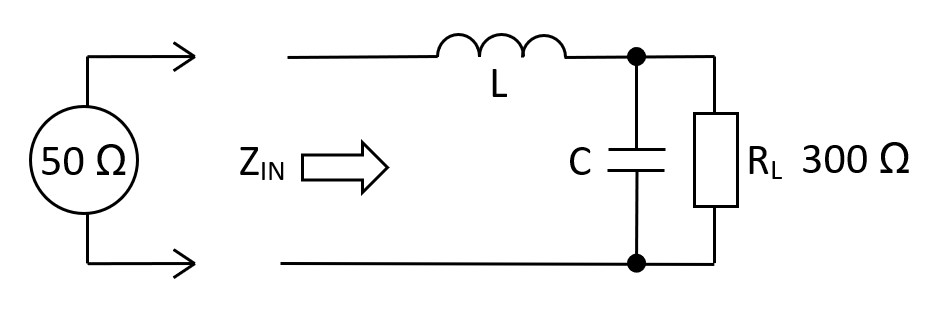
- # Low-pass simulation
- **Circuit**
- 
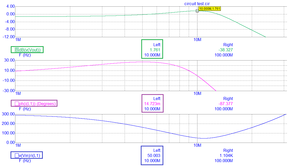
- **Results**
- 
- **Conclusion**
- What the results tell us at 10 MHz is this: -
- - The voltage amplification to the load from the source is 1.761 dB
- - A 50 Ω to 50 Ω interface will naturally attenuate by 6 dB hence, the result is good
- - The phase angle of current into L1 is leading the applied voltage by a fraction of 1 degree (0.0147°) i.e. the circuit input impedance can be regarded as resistive
- - The input impedance magnitude is 50.003 Ω i.e. as desired
- - The usable bandwidth (± 10°) is about 2 MHz producing a 63 Ω to 46 Ω impedance magnitude change across the bandwidth
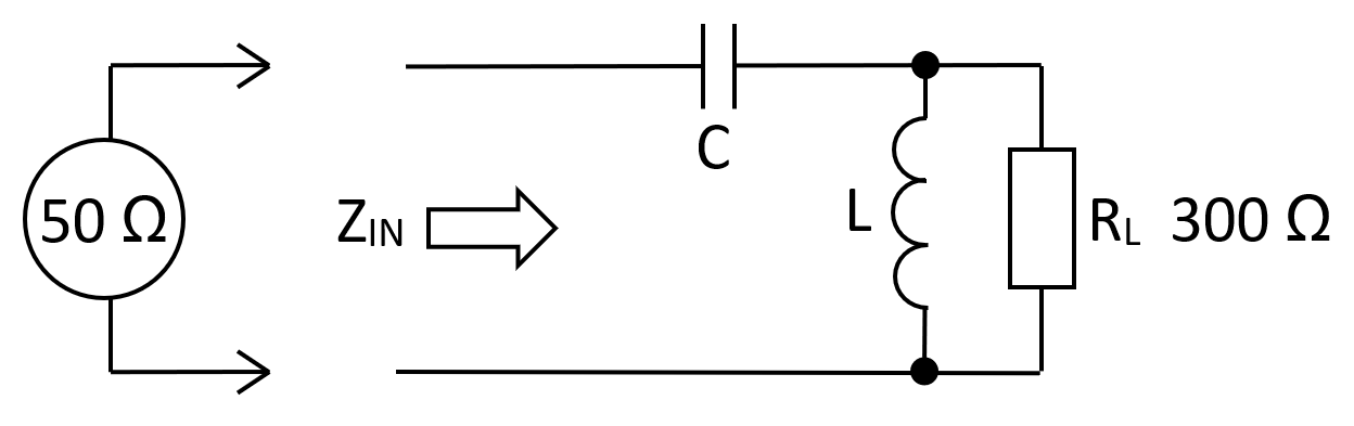
- # High-pass impedance transformation
- The alternative to the above circuit is to swap L and C like this: -
- 
- Without going through the math again we get: -
- $$\boxed{R_{IN} = \dfrac{L}{R_L C}} \text{ and therefore } \boxed{L = R_{IN} R_L C}\text{ (as previously) but,}$$
- $$\boxed{ C = \dfrac{1}{\omega R_{IN}}\sqrt{\dfrac{1}{\dfrac{R_L}{R_{IN}}-1}} }$$
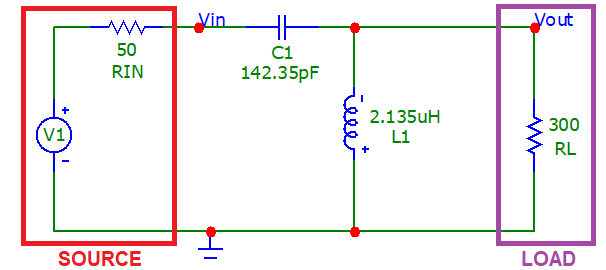
- So, if the frequency is 10 MHz, **C = 142.35 pF**
- Given C, we can calculate **L = 2.135 μH** and we see this AC response: -
- # High-pass simulation
- 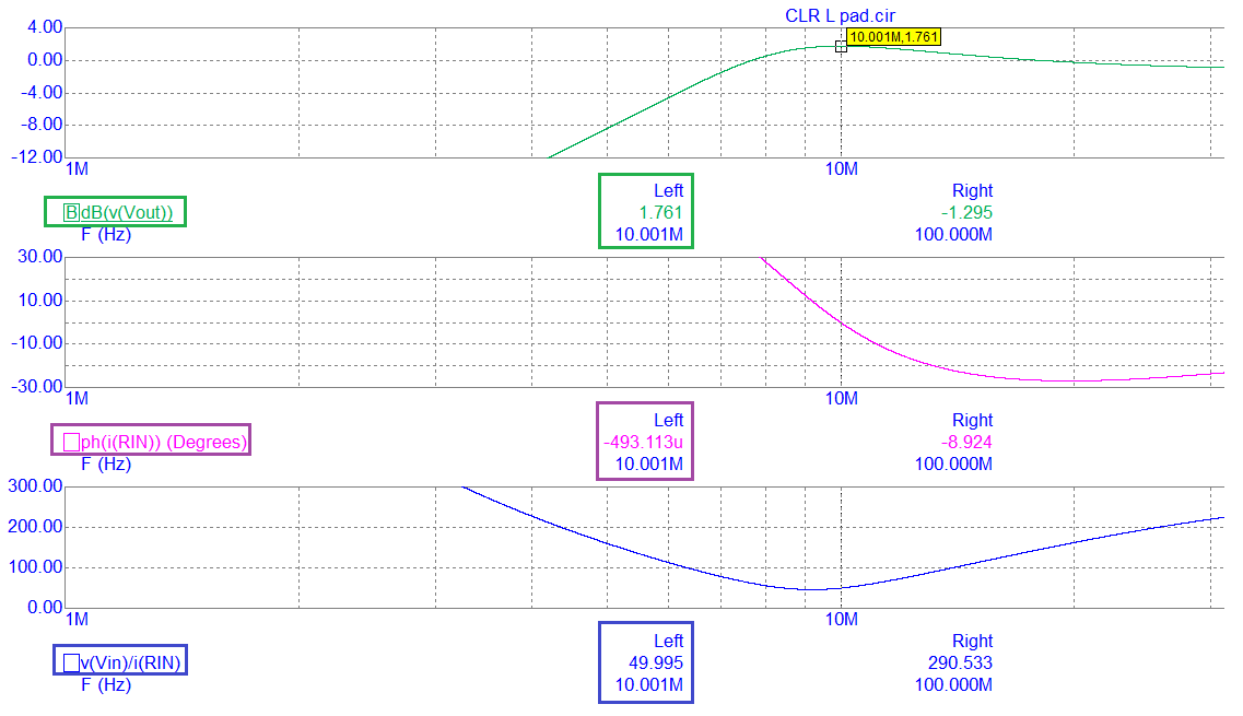
- **Conclusion**
- - The voltage amplification is 1.761 dB (as per low-pass version)
- - The phase angle of current into L1 is leading the applied voltage by a fraction of 1 degree (0.000493°) i.e. the circuit input impedance can be regarded as resistive
- - The input impedance magnitude is 49.995 Ω i.e. as desired
- # Why choose one over the other?
- Both circuits work just fine for resistive loads but, if the load is partially reactive (as is often the case), the load can be broken into its parallel equivalent circuit. Then, you choose the top circuit for a load that has parallel capacitance and, you choose the lower circuit for a load that has parallel inductance. Then make the appropriate numerical adjustments to C (low-pass) or L (high-pass).
- # Low-pass impedance transformation
- 
- # Theory
- Input Impedance: -
- $$Z_{IN} = j\omega L + \dfrac{\dfrac{R_L}{j\omega C}}{R_L + \dfrac{1}{j\omega C}} = j\omega L +\dfrac{R_L}{1 + j\omega R_L C} = \dfrac{j\omega L - \omega^2 R_L LC + R_L}{1 + j\omega R_L C}$$
- Multiply numerator and denominator by the denominator's complex conjugate to get: -
- $$Z_{IN} = \dfrac{(j\omega L - \omega^2 R_L LC + R_L)(1 - j\omega R_L C)}{1 + \omega^2 R_L^2 C^2}$$
- $$Z_{IN} = \dfrac{j\omega L -\omega^2 R_L LC + R_L + \omega^2 R_L LC +j\omega^3 R_L^2 LC^2 - j\omega R_L^2 C}{1 + \omega^2 R_L^2 C^2}$$
- $$\boxed{Z_{IN} = \dfrac{j\omega L + R_L + j\omega^3 R_L^2 LC^2 - j\omega R_L^2 C}{1 + \omega^2 R_L^2 C^2}}$$
- To find \$\color{red}{\boxed{\omega}}\$ that produces a real impedance, equate the numerator's imaginary terms to zero: -
- $$\omega L + \omega^3 R_L^2 LC^2 - \omega R_L^2 C = 0$$
- $$\color{red}{\boxed{\omega = \sqrt{\dfrac{R_L^2 C - L}{R_L^2 LC^2}} = \sqrt{\dfrac{1}{LC} - \dfrac{1}{R_L^2 C^2}}}}$$
- \$\color{red}{\boxed{\omega}}\$ is the operating frequency of the impedance transformer. We use this relationship below: -
- -----
- With imaginary terms at zero, \$Z_{IN}\rightarrow R_{IN}\$ hence: -
- $$\boxed{R_{IN} = \dfrac{\cancel{j\omega L} + R_L + \cancel{j\omega^3 R_L^2 LC^2} - \cancel{j\omega R_L^2 C}}{1 + \omega^2 R_L^2 C^2}} = \dfrac{R_L}{1 + \omega^2 R_L^2 C^2}$$
- If we substitute the formula for \$\color{red}{\boxed{\omega}}\$ in the above equation, we can drill down to this: -
- $$\boxed{R_{IN} = \dfrac{L}{R_L C}} \text{ and therefore } \boxed{L = R_{IN} R_L C}$$
- We can now substitute for L in the \$\color{red}{\boxed{\omega}}\$ equation hence: -
- $$\color{red}{\omega = \sqrt{\dfrac{1}{LC} - \dfrac{1}{R_L^2 C^2}}}\color{black}{ \Longrightarrow \dfrac{1}{C}\sqrt{\dfrac{1}{R_{IN} R_L} - \dfrac{1}{R_L^2}} = \dfrac{1}{R_L C}\sqrt{\dfrac{R_L}{R_{IN}}-1}}$$
- We can now solve for C: -
- $$\boxed{ C = \dfrac{1}{\omega R_L}\sqrt{\dfrac{R_L}{R_{IN}}-1} }$$
- So, if the frequency is 10 MHz, **C = 118.62 pF**
- Given C, we can calculate **L = 1.779 μH**
- # Low-pass simulation
- **Circuit**
- 
- **Results**
- 
- **Conclusion**
- What the results tell us at 10 MHz is this: -
- - The voltage amplification to the load from the source is 1.761 dB
- - A 50 Ω to 50 Ω interface will naturally attenuate by 6 dB hence, the result is good
- - The phase angle of current into L1 is leading the applied voltage by a fraction of 1 degree (0.0147°) i.e. the circuit input impedance can be regarded as resistive
- - The input impedance magnitude is 50.003 Ω i.e. as desired
- - The usable bandwidth (± 10°) is about 2 MHz producing a 63 Ω to 46 Ω impedance magnitude change across the bandwidth
- # High-pass impedance transformation
- The alternative to the above circuit is to swap L and C like this: -
- 
- Without going through the math again we get: -
- $$\boxed{R_{IN} = \dfrac{L}{R_L C}} \text{ and therefore } \boxed{L = R_{IN} R_L C}\text{ (as previously) but,}$$
- $$\boxed{ C = \dfrac{1}{\omega R_{IN}}\sqrt{\dfrac{1}{\dfrac{R_L}{R_{IN}}-1}} }$$
- So, if the frequency is 10 MHz, **C = 142.35 pF**
- Given C, we can calculate **L = 2.135 μH** and we see this AC response: -
- # High-pass simulation
- **Circuit**
- 
- **Results**
- 
- **Conclusion**
- - The voltage amplification is 1.761 dB (as per low-pass version)
- - The phase angle of current into L1 is leading the applied voltage by a fraction of 1 degree (0.000493°) i.e. the circuit input impedance can be regarded as resistive
- - The input impedance magnitude is 49.995 Ω i.e. as desired
- # Why choose one over the other?
- Both circuits work just fine for resistive loads but, if the load is partially reactive (as is often the case), the load can be broken into its parallel equivalent circuit. Then, you choose the top circuit for a load that has parallel capacitance and, you choose the lower circuit for a load that has parallel inductance. Then make the appropriate numerical adjustments to C (low-pass) or L (high-pass).
#13: Post edited
by
Andy aka
·
2020-06-25T12:10:17Z (almost 5 years ago)
- # Low-pass impedance transformation
- 
- # Theory
Impedance \$Z_{IN}\$ is: -$$j\omega L + \dfrac{\dfrac{R_L}{j\omega C}}{R_L + \dfrac{1}{j\omega C}} = j\omega L +\dfrac{R_L}{1 + j\omega R_L C} = \dfrac{j\omega L - \omega^2 R_L LC + R_L}{1 + j\omega R_L C}$$- Multiply numerator and denominator by the denominator's complex conjugate to get: -
- $$Z_{IN} = \dfrac{(j\omega L - \omega^2 R_L LC + R_L)(1 - j\omega R_L C)}{1 + \omega^2 R_L^2 C^2}$$
- $$Z_{IN} = \dfrac{j\omega L -\omega^2 R_L LC + R_L + \omega^2 R_L LC +j\omega^3 R_L^2 LC^2 - j\omega R_L^2 C}{1 + \omega^2 R_L^2 C^2}$$
$$Z_{IN} = \dfrac{j\omega L + R_L + j\omega^3 R_L^2 LC^2 - j\omega R_L^2 C}{1 + \omega^2 R_L^2 C^2}$$- To find \$\color{red}{\boxed{\omega}}\$ that produces a real impedance, equate the numerator's imaginary terms to zero: -
- $$\omega L + \omega^3 R_L^2 LC^2 - \omega R_L^2 C = 0$$
- $$\color{red}{\boxed{\omega = \sqrt{\dfrac{R_L^2 C - L}{R_L^2 LC^2}} = \sqrt{\dfrac{1}{LC} - \dfrac{1}{R_L^2 C^2}}}}$$
\$\color{red}{\boxed{\omega}}\$ is the operating frequency for the transformation.- -----
- With imaginary terms at zero, \$Z_{IN}\rightarrow R_{IN}\$ hence: -
$$R_{IN} = \dfrac{R_L}{1 + \omega^2 R_L^2 C^2}$$- If we substitute the formula for \$\color{red}{\boxed{\omega}}\$ in the above equation, we can drill down to this: -
- $$\boxed{R_{IN} = \dfrac{L}{R_L C}} \text{ and therefore } \boxed{L = R_{IN} R_L C}$$
- We can now substitute for L in the \$\color{red}{\boxed{\omega}}\$ equation hence: -
- $$\color{red}{\omega = \sqrt{\dfrac{1}{LC} - \dfrac{1}{R_L^2 C^2}}}\color{black}{ \Longrightarrow \dfrac{1}{C}\sqrt{\dfrac{1}{R_{IN} R_L} - \dfrac{1}{R_L^2}} = \dfrac{1}{R_L C}\sqrt{\dfrac{R_L}{R_{IN}}-1}}$$
- We can now solve for C: -
- $$\boxed{ C = \dfrac{1}{\omega R_L}\sqrt{\dfrac{R_L}{R_{IN}}-1} }$$
- So, if the frequency is 10 MHz, **C = 118.62 pF**
- Given C, we can calculate **L = 1.779 μH**
- # Low-pass simulation
- **Circuit**
- 
- **Results**
- 
- **Conclusion**
- What the results tell us at 10 MHz is this: -
- - The voltage amplification to the load from the source is 1.761 dB
- - A 50 Ω to 50 Ω interface will naturally attenuate by 6 dB hence, the result is good
- - The phase angle of current into L1 is leading the applied voltage by a fraction of 1 degree (0.0147°) i.e. the circuit input impedance can be regarded as resistive
- - The input impedance magnitude is 50.003 Ω i.e. as desired
- - The usable bandwidth (± 10°) is about 2 MHz producing a 63 Ω to 46 Ω impedance magnitude change across the bandwidth
- # High-pass impedance transformation
- The alternative to the above circuit is to swap L and C like this: -
- 
- Without going through the math again we get: -
- $$\boxed{R_{IN} = \dfrac{L}{R_L C}} \text{ and therefore } \boxed{L = R_{IN} R_L C}\text{ (as previously) but,}$$
- $$\boxed{ C = \dfrac{1}{\omega R_{IN}}\sqrt{\dfrac{1}{\dfrac{R_L}{R_{IN}}-1}} }$$
- So, if the frequency is 10 MHz, **C = 142.35 pF**
- Given C, we can calculate **L = 2.135 μH** and we see this AC response: -
- # High-pass simulation
- # Why choose one over the other?
- Both circuits work just fine for resistive loads but, if the load is partially reactive (as is often the case), the load can be broken into its parallel equivalent circuit. Then, you choose the top circuit for a load that has parallel capacitance and, you choose the lower circuit for a load that has parallel inductance. Then make the appropriate numerical adjustments to C (low-pass) or L (high-pass).
- # Low-pass impedance transformation
- 
- # Theory
- Input Impedance: -
- $$Z_{IN} = j\omega L + \dfrac{\dfrac{R_L}{j\omega C}}{R_L + \dfrac{1}{j\omega C}} = j\omega L +\dfrac{R_L}{1 + j\omega R_L C} = \dfrac{j\omega L - \omega^2 R_L LC + R_L}{1 + j\omega R_L C}$$
- Multiply numerator and denominator by the denominator's complex conjugate to get: -
- $$Z_{IN} = \dfrac{(j\omega L - \omega^2 R_L LC + R_L)(1 - j\omega R_L C)}{1 + \omega^2 R_L^2 C^2}$$
- $$Z_{IN} = \dfrac{j\omega L -\omega^2 R_L LC + R_L + \omega^2 R_L LC +j\omega^3 R_L^2 LC^2 - j\omega R_L^2 C}{1 + \omega^2 R_L^2 C^2}$$
- $$\boxed{Z_{IN} = \dfrac{j\omega L + R_L + j\omega^3 R_L^2 LC^2 - j\omega R_L^2 C}{1 + \omega^2 R_L^2 C^2}}$$
- To find \$\color{red}{\boxed{\omega}}\$ that produces a real impedance, equate the numerator's imaginary terms to zero: -
- $$\omega L + \omega^3 R_L^2 LC^2 - \omega R_L^2 C = 0$$
- $$\color{red}{\boxed{\omega = \sqrt{\dfrac{R_L^2 C - L}{R_L^2 LC^2}} = \sqrt{\dfrac{1}{LC} - \dfrac{1}{R_L^2 C^2}}}}$$
- \$\color{red}{\boxed{\omega}}\$ is the operating frequency of the impedance transformer. We use this relationship below: -
- -----
- With imaginary terms at zero, \$Z_{IN}\rightarrow R_{IN}\$ hence: -
- $$\boxed{R_{IN} = \dfrac{\cancel{j\omega L} + R_L + \cancel{j\omega^3 R_L^2 LC^2} - \cancel{j\omega R_L^2 C}}{1 + \omega^2 R_L^2 C^2}} = \dfrac{R_L}{1 + \omega^2 R_L^2 C^2}$$
- If we substitute the formula for \$\color{red}{\boxed{\omega}}\$ in the above equation, we can drill down to this: -
- $$\boxed{R_{IN} = \dfrac{L}{R_L C}} \text{ and therefore } \boxed{L = R_{IN} R_L C}$$
- We can now substitute for L in the \$\color{red}{\boxed{\omega}}\$ equation hence: -
- $$\color{red}{\omega = \sqrt{\dfrac{1}{LC} - \dfrac{1}{R_L^2 C^2}}}\color{black}{ \Longrightarrow \dfrac{1}{C}\sqrt{\dfrac{1}{R_{IN} R_L} - \dfrac{1}{R_L^2}} = \dfrac{1}{R_L C}\sqrt{\dfrac{R_L}{R_{IN}}-1}}$$
- We can now solve for C: -
- $$\boxed{ C = \dfrac{1}{\omega R_L}\sqrt{\dfrac{R_L}{R_{IN}}-1} }$$
- So, if the frequency is 10 MHz, **C = 118.62 pF**
- Given C, we can calculate **L = 1.779 μH**
- # Low-pass simulation
- **Circuit**
- 
- **Results**
- 
- **Conclusion**
- What the results tell us at 10 MHz is this: -
- - The voltage amplification to the load from the source is 1.761 dB
- - A 50 Ω to 50 Ω interface will naturally attenuate by 6 dB hence, the result is good
- - The phase angle of current into L1 is leading the applied voltage by a fraction of 1 degree (0.0147°) i.e. the circuit input impedance can be regarded as resistive
- - The input impedance magnitude is 50.003 Ω i.e. as desired
- - The usable bandwidth (± 10°) is about 2 MHz producing a 63 Ω to 46 Ω impedance magnitude change across the bandwidth
- # High-pass impedance transformation
- The alternative to the above circuit is to swap L and C like this: -
- 
- Without going through the math again we get: -
- $$\boxed{R_{IN} = \dfrac{L}{R_L C}} \text{ and therefore } \boxed{L = R_{IN} R_L C}\text{ (as previously) but,}$$
- $$\boxed{ C = \dfrac{1}{\omega R_{IN}}\sqrt{\dfrac{1}{\dfrac{R_L}{R_{IN}}-1}} }$$
- So, if the frequency is 10 MHz, **C = 142.35 pF**
- Given C, we can calculate **L = 2.135 μH** and we see this AC response: -
- # High-pass simulation
- 
- **Conclusion**
- - The voltage amplification is 1.761 dB (as per low-pass version)
- - The phase angle of current into L1 is leading the applied voltage by a fraction of 1 degree (0.000493°) i.e. the circuit input impedance can be regarded as resistive
- - The input impedance magnitude is 49.995 Ω i.e. as desired
- # Why choose one over the other?
- Both circuits work just fine for resistive loads but, if the load is partially reactive (as is often the case), the load can be broken into its parallel equivalent circuit. Then, you choose the top circuit for a load that has parallel capacitance and, you choose the lower circuit for a load that has parallel inductance. Then make the appropriate numerical adjustments to C (low-pass) or L (high-pass).
#12: Post edited
by
Andy aka
·
2020-06-24T15:25:23Z (almost 5 years ago)
- # Low-pass impedance transformation
- 
- # Theory
- Impedance \$Z_{IN}\$ is: -
- $$j\omega L + \dfrac{\dfrac{R_L}{j\omega C}}{R_L + \dfrac{1}{j\omega C}} = j\omega L +\dfrac{R_L}{1 + j\omega R_L C} = \dfrac{j\omega L - \omega^2 R_L LC + R_L}{1 + j\omega R_L C}$$
- Multiply numerator and denominator by the denominator's complex conjugate to get: -
- $$Z_{IN} = \dfrac{(j\omega L - \omega^2 R_L LC + R_L)(1 - j\omega R_L C)}{1 + \omega^2 R_L^2 C^2}$$
- $$Z_{IN} = \dfrac{j\omega L -\omega^2 R_L LC + R_L + \omega^2 R_L LC +j\omega^3 R_L^2 LC^2 - j\omega R_L^2 C}{1 + \omega^2 R_L^2 C^2}$$
- $$Z_{IN} = \dfrac{j\omega L + R_L + j\omega^3 R_L^2 LC^2 - j\omega R_L^2 C}{1 + \omega^2 R_L^2 C^2}$$
- To find \$\color{red}{\boxed{\omega}}\$ that produces a real impedance, equate the numerator's imaginary terms to zero: -
- $$\omega L + \omega^3 R_L^2 LC^2 - \omega R_L^2 C = 0$$
- $$\color{red}{\boxed{\omega = \sqrt{\dfrac{R_L^2 C - L}{R_L^2 LC^2}} = \sqrt{\dfrac{1}{LC} - \dfrac{1}{R_L^2 C^2}}}}$$
- \$\color{red}{\boxed{\omega}}\$ is the operating frequency for the transformation.
- -----
- With imaginary terms at zero, \$Z_{IN}\rightarrow R_{IN}\$ hence: -
- $$R_{IN} = \dfrac{R_L}{1 + \omega^2 R_L^2 C^2}$$
- If we substitute the formula for \$\color{red}{\boxed{\omega}}\$ in the above equation, we can drill down to this: -
- $$\boxed{R_{IN} = \dfrac{L}{R_L C}} \text{ and therefore } \boxed{L = R_{IN} R_L C}$$
- We can now substitute for L in the \$\color{red}{\boxed{\omega}}\$ equation hence: -
- $$\color{red}{\omega = \sqrt{\dfrac{1}{LC} - \dfrac{1}{R_L^2 C^2}}}\color{black}{ \Longrightarrow \dfrac{1}{C}\sqrt{\dfrac{1}{R_{IN} R_L} - \dfrac{1}{R_L^2}} = \dfrac{1}{R_L C}\sqrt{\dfrac{R_L}{R_{IN}}-1}}$$
- We can now solve for C: -
- $$\boxed{ C = \dfrac{1}{\omega R_L}\sqrt{\dfrac{R_L}{R_{IN}}-1} }$$
- So, if the frequency is 10 MHz, **C = 118.62 pF**
- Given C, we can calculate **L = 1.779 μH**
- # Low-pass simulation
- **Circuit**
- 
- **Results**
- **Conclusion**
- What the results tell us at 10 MHz is this: -
- - The voltage amplification to the load from the source is 1.761 dB
- - A 50 Ω to 50 Ω interface will naturally attenuate by 6 dB hence, the result is good
- - The phase angle of current into L1 is leading the applied voltage by a fraction of 1 degree (0.0147°) i.e. the circuit input impedance can be regarded as resistive
- - The input impedance magnitude is 50.003 Ω i.e. as desired
- - The usable bandwidth (± 10°) is about 2 MHz producing a 63 Ω to 46 Ω impedance magnitude change across the bandwidth
- # High-pass impedance transformation
- The alternative to the above circuit is to swap L and C like this: -
- 
- Without going through the math again we get: -
- $$\boxed{R_{IN} = \dfrac{L}{R_L C}} \text{ and therefore } \boxed{L = R_{IN} R_L C}\text{ (as previously) but,}$$
- $$\boxed{ C = \dfrac{1}{\omega R_{IN}}\sqrt{\dfrac{1}{\dfrac{R_L}{R_{IN}}-1}} }$$
- So, if the frequency is 10 MHz, **C = 142.35 pF**
- Given C, we can calculate **L = 2.135 μH** and we see this AC response: -
- # High-pass simulation
- # Why choose one over the other?
- Both circuits work just fine for resistive loads but, if the load is partially reactive (as is often the case), the load can be broken into its parallel equivalent circuit. Then, you choose the top circuit for a load that has parallel capacitance and, you choose the lower circuit for a load that has parallel inductance. Then make the appropriate numerical adjustments to C (low-pass) or L (high-pass).
- # Low-pass impedance transformation
- 
- # Theory
- Impedance \$Z_{IN}\$ is: -
- $$j\omega L + \dfrac{\dfrac{R_L}{j\omega C}}{R_L + \dfrac{1}{j\omega C}} = j\omega L +\dfrac{R_L}{1 + j\omega R_L C} = \dfrac{j\omega L - \omega^2 R_L LC + R_L}{1 + j\omega R_L C}$$
- Multiply numerator and denominator by the denominator's complex conjugate to get: -
- $$Z_{IN} = \dfrac{(j\omega L - \omega^2 R_L LC + R_L)(1 - j\omega R_L C)}{1 + \omega^2 R_L^2 C^2}$$
- $$Z_{IN} = \dfrac{j\omega L -\omega^2 R_L LC + R_L + \omega^2 R_L LC +j\omega^3 R_L^2 LC^2 - j\omega R_L^2 C}{1 + \omega^2 R_L^2 C^2}$$
- $$Z_{IN} = \dfrac{j\omega L + R_L + j\omega^3 R_L^2 LC^2 - j\omega R_L^2 C}{1 + \omega^2 R_L^2 C^2}$$
- To find \$\color{red}{\boxed{\omega}}\$ that produces a real impedance, equate the numerator's imaginary terms to zero: -
- $$\omega L + \omega^3 R_L^2 LC^2 - \omega R_L^2 C = 0$$
- $$\color{red}{\boxed{\omega = \sqrt{\dfrac{R_L^2 C - L}{R_L^2 LC^2}} = \sqrt{\dfrac{1}{LC} - \dfrac{1}{R_L^2 C^2}}}}$$
- \$\color{red}{\boxed{\omega}}\$ is the operating frequency for the transformation.
- -----
- With imaginary terms at zero, \$Z_{IN}\rightarrow R_{IN}\$ hence: -
- $$R_{IN} = \dfrac{R_L}{1 + \omega^2 R_L^2 C^2}$$
- If we substitute the formula for \$\color{red}{\boxed{\omega}}\$ in the above equation, we can drill down to this: -
- $$\boxed{R_{IN} = \dfrac{L}{R_L C}} \text{ and therefore } \boxed{L = R_{IN} R_L C}$$
- We can now substitute for L in the \$\color{red}{\boxed{\omega}}\$ equation hence: -
- $$\color{red}{\omega = \sqrt{\dfrac{1}{LC} - \dfrac{1}{R_L^2 C^2}}}\color{black}{ \Longrightarrow \dfrac{1}{C}\sqrt{\dfrac{1}{R_{IN} R_L} - \dfrac{1}{R_L^2}} = \dfrac{1}{R_L C}\sqrt{\dfrac{R_L}{R_{IN}}-1}}$$
- We can now solve for C: -
- $$\boxed{ C = \dfrac{1}{\omega R_L}\sqrt{\dfrac{R_L}{R_{IN}}-1} }$$
- So, if the frequency is 10 MHz, **C = 118.62 pF**
- Given C, we can calculate **L = 1.779 μH**
- # Low-pass simulation
- **Circuit**
- 
- **Results**
- 
- **Conclusion**
- What the results tell us at 10 MHz is this: -
- - The voltage amplification to the load from the source is 1.761 dB
- - A 50 Ω to 50 Ω interface will naturally attenuate by 6 dB hence, the result is good
- - The phase angle of current into L1 is leading the applied voltage by a fraction of 1 degree (0.0147°) i.e. the circuit input impedance can be regarded as resistive
- - The input impedance magnitude is 50.003 Ω i.e. as desired
- - The usable bandwidth (± 10°) is about 2 MHz producing a 63 Ω to 46 Ω impedance magnitude change across the bandwidth
- # High-pass impedance transformation
- The alternative to the above circuit is to swap L and C like this: -
- 
- Without going through the math again we get: -
- $$\boxed{R_{IN} = \dfrac{L}{R_L C}} \text{ and therefore } \boxed{L = R_{IN} R_L C}\text{ (as previously) but,}$$
- $$\boxed{ C = \dfrac{1}{\omega R_{IN}}\sqrt{\dfrac{1}{\dfrac{R_L}{R_{IN}}-1}} }$$
- So, if the frequency is 10 MHz, **C = 142.35 pF**
- Given C, we can calculate **L = 2.135 μH** and we see this AC response: -
- # High-pass simulation
- 
- # Why choose one over the other?
- Both circuits work just fine for resistive loads but, if the load is partially reactive (as is often the case), the load can be broken into its parallel equivalent circuit. Then, you choose the top circuit for a load that has parallel capacitance and, you choose the lower circuit for a load that has parallel inductance. Then make the appropriate numerical adjustments to C (low-pass) or L (high-pass).
#11: Post edited
by
Andy aka
·
2020-06-24T13:20:53Z (almost 5 years ago)
# Schematic 1 - low-pass- 
- # Theory
- Impedance \$Z_{IN}\$ is: -
- $$j\omega L + \dfrac{\dfrac{R_L}{j\omega C}}{R_L + \dfrac{1}{j\omega C}} = j\omega L +\dfrac{R_L}{1 + j\omega R_L C} = \dfrac{j\omega L - \omega^2 R_L LC + R_L}{1 + j\omega R_L C}$$
- Multiply numerator and denominator by the denominator's complex conjugate to get: -
- $$Z_{IN} = \dfrac{(j\omega L - \omega^2 R_L LC + R_L)(1 - j\omega R_L C)}{1 + \omega^2 R_L^2 C^2}$$
- $$Z_{IN} = \dfrac{j\omega L -\omega^2 R_L LC + R_L + \omega^2 R_L LC +j\omega^3 R_L^2 LC^2 - j\omega R_L^2 C}{1 + \omega^2 R_L^2 C^2}$$
- $$Z_{IN} = \dfrac{j\omega L + R_L + j\omega^3 R_L^2 LC^2 - j\omega R_L^2 C}{1 + \omega^2 R_L^2 C^2}$$
- To find \$\color{red}{\boxed{\omega}}\$ that produces a real impedance, equate the numerator's imaginary terms to zero: -
- $$\omega L + \omega^3 R_L^2 LC^2 - \omega R_L^2 C = 0$$
- $$\color{red}{\boxed{\omega = \sqrt{\dfrac{R_L^2 C - L}{R_L^2 LC^2}} = \sqrt{\dfrac{1}{LC} - \dfrac{1}{R_L^2 C^2}}}}$$
- \$\color{red}{\boxed{\omega}}\$ is the operating frequency for the transformation.
- -----
- With imaginary terms at zero, \$Z_{IN}\rightarrow R_{IN}\$ hence: -
- $$R_{IN} = \dfrac{R_L}{1 + \omega^2 R_L^2 C^2}$$
- If we substitute the formula for \$\color{red}{\boxed{\omega}}\$ in the above equation, we can drill down to this: -
- $$\boxed{R_{IN} = \dfrac{L}{R_L C}} \text{ and therefore } \boxed{L = R_{IN} R_L C}$$
- We can now substitute for L in the \$\color{red}{\boxed{\omega}}\$ equation hence: -
- $$\color{red}{\omega = \sqrt{\dfrac{1}{LC} - \dfrac{1}{R_L^2 C^2}}}\color{black}{ \Longrightarrow \dfrac{1}{C}\sqrt{\dfrac{1}{R_{IN} R_L} - \dfrac{1}{R_L^2}} = \dfrac{1}{R_L C}\sqrt{\dfrac{R_L}{R_{IN}}-1}}$$
- We can now solve for C: -
- $$\boxed{ C = \dfrac{1}{\omega R_L}\sqrt{\dfrac{R_L}{R_{IN}}-1} }$$
- So, if the frequency is 10 MHz, **C = 118.62 pF**
- Given C, we can calculate **L = 1.779 μH**
# Simulation 1- **Circuit**
- 
- **Results**
- 
- **Conclusion**
- What the results tell us at 10 MHz is this: -
- - The voltage amplification to the load from the source is 1.761 dB
- - A 50 Ω to 50 Ω interface will naturally attenuate by 6 dB hence, the result is good
- - The phase angle of current into L1 is leading the applied voltage by a fraction of 1 degree (0.0147°) i.e. the circuit input impedance can be regarded as resistive
- - The input impedance magnitude is 50.003 Ω i.e. as desired
- - The usable bandwidth (± 10°) is about 2 MHz producing a 63 Ω to 46 Ω impedance magnitude change across the bandwidth
# Schematic 2 - high-pass- The alternative to the above circuit is to swap L and C like this: -
- 
- Without going through the math again we get: -
- $$\boxed{R_{IN} = \dfrac{L}{R_L C}} \text{ and therefore } \boxed{L = R_{IN} R_L C}\text{ (as previously) but,}$$
- $$\boxed{ C = \dfrac{1}{\omega R_{IN}}\sqrt{\dfrac{1}{\dfrac{R_L}{R_{IN}}-1}} }$$
- So, if the frequency is 10 MHz, **C = 142.35 pF**
Given C, we can calculate **L = 2.135 μH** and we see: -- 
- # Why choose one over the other?
- Both circuits work just fine for resistive loads but, if the load is partially reactive (as is often the case), the load can be broken into its parallel equivalent circuit. Then, you choose the top circuit for a load that has parallel capacitance and, you choose the lower circuit for a load that has parallel inductance. Then make the appropriate numerical adjustments to C (low-pass) or L (high-pass).
- # Low-pass impedance transformation
- 
- # Theory
- Impedance \$Z_{IN}\$ is: -
- $$j\omega L + \dfrac{\dfrac{R_L}{j\omega C}}{R_L + \dfrac{1}{j\omega C}} = j\omega L +\dfrac{R_L}{1 + j\omega R_L C} = \dfrac{j\omega L - \omega^2 R_L LC + R_L}{1 + j\omega R_L C}$$
- Multiply numerator and denominator by the denominator's complex conjugate to get: -
- $$Z_{IN} = \dfrac{(j\omega L - \omega^2 R_L LC + R_L)(1 - j\omega R_L C)}{1 + \omega^2 R_L^2 C^2}$$
- $$Z_{IN} = \dfrac{j\omega L -\omega^2 R_L LC + R_L + \omega^2 R_L LC +j\omega^3 R_L^2 LC^2 - j\omega R_L^2 C}{1 + \omega^2 R_L^2 C^2}$$
- $$Z_{IN} = \dfrac{j\omega L + R_L + j\omega^3 R_L^2 LC^2 - j\omega R_L^2 C}{1 + \omega^2 R_L^2 C^2}$$
- To find \$\color{red}{\boxed{\omega}}\$ that produces a real impedance, equate the numerator's imaginary terms to zero: -
- $$\omega L + \omega^3 R_L^2 LC^2 - \omega R_L^2 C = 0$$
- $$\color{red}{\boxed{\omega = \sqrt{\dfrac{R_L^2 C - L}{R_L^2 LC^2}} = \sqrt{\dfrac{1}{LC} - \dfrac{1}{R_L^2 C^2}}}}$$
- \$\color{red}{\boxed{\omega}}\$ is the operating frequency for the transformation.
- -----
- With imaginary terms at zero, \$Z_{IN}\rightarrow R_{IN}\$ hence: -
- $$R_{IN} = \dfrac{R_L}{1 + \omega^2 R_L^2 C^2}$$
- If we substitute the formula for \$\color{red}{\boxed{\omega}}\$ in the above equation, we can drill down to this: -
- $$\boxed{R_{IN} = \dfrac{L}{R_L C}} \text{ and therefore } \boxed{L = R_{IN} R_L C}$$
- We can now substitute for L in the \$\color{red}{\boxed{\omega}}\$ equation hence: -
- $$\color{red}{\omega = \sqrt{\dfrac{1}{LC} - \dfrac{1}{R_L^2 C^2}}}\color{black}{ \Longrightarrow \dfrac{1}{C}\sqrt{\dfrac{1}{R_{IN} R_L} - \dfrac{1}{R_L^2}} = \dfrac{1}{R_L C}\sqrt{\dfrac{R_L}{R_{IN}}-1}}$$
- We can now solve for C: -
- $$\boxed{ C = \dfrac{1}{\omega R_L}\sqrt{\dfrac{R_L}{R_{IN}}-1} }$$
- So, if the frequency is 10 MHz, **C = 118.62 pF**
- Given C, we can calculate **L = 1.779 μH**
- # Low-pass simulation
- **Circuit**
- 
- **Results**
- 
- **Conclusion**
- What the results tell us at 10 MHz is this: -
- - The voltage amplification to the load from the source is 1.761 dB
- - A 50 Ω to 50 Ω interface will naturally attenuate by 6 dB hence, the result is good
- - The phase angle of current into L1 is leading the applied voltage by a fraction of 1 degree (0.0147°) i.e. the circuit input impedance can be regarded as resistive
- - The input impedance magnitude is 50.003 Ω i.e. as desired
- - The usable bandwidth (± 10°) is about 2 MHz producing a 63 Ω to 46 Ω impedance magnitude change across the bandwidth
- # High-pass impedance transformation
- The alternative to the above circuit is to swap L and C like this: -
- 
- Without going through the math again we get: -
- $$\boxed{R_{IN} = \dfrac{L}{R_L C}} \text{ and therefore } \boxed{L = R_{IN} R_L C}\text{ (as previously) but,}$$
- $$\boxed{ C = \dfrac{1}{\omega R_{IN}}\sqrt{\dfrac{1}{\dfrac{R_L}{R_{IN}}-1}} }$$
- So, if the frequency is 10 MHz, **C = 142.35 pF**
- Given C, we can calculate **L = 2.135 μH** and we see this AC response: -
- # High-pass simulation
- 
- # Why choose one over the other?
- Both circuits work just fine for resistive loads but, if the load is partially reactive (as is often the case), the load can be broken into its parallel equivalent circuit. Then, you choose the top circuit for a load that has parallel capacitance and, you choose the lower circuit for a load that has parallel inductance. Then make the appropriate numerical adjustments to C (low-pass) or L (high-pass).
#10: Post edited
by
Andy aka
·
2020-06-24T13:16:48Z (almost 5 years ago)
- # Schematic 1 - low-pass
- 
- # Theory
- Impedance \$Z_{IN}\$ is: -
- $$j\omega L + \dfrac{\dfrac{R_L}{j\omega C}}{R_L + \dfrac{1}{j\omega C}} = j\omega L +\dfrac{R_L}{1 + j\omega R_L C} = \dfrac{j\omega L - \omega^2 R_L LC + R_L}{1 + j\omega R_L C}$$
- Multiply numerator and denominator by the denominator's complex conjugate to get: -
- $$Z_{IN} = \dfrac{(j\omega L - \omega^2 R_L LC + R_L)(1 - j\omega R_L C)}{1 + \omega^2 R_L^2 C^2}$$
- $$Z_{IN} = \dfrac{j\omega L -\omega^2 R_L LC + R_L + \omega^2 R_L LC +j\omega^3 R_L^2 LC^2 - j\omega R_L^2 C}{1 + \omega^2 R_L^2 C^2}$$
- $$Z_{IN} = \dfrac{j\omega L + R_L + j\omega^3 R_L^2 LC^2 - j\omega R_L^2 C}{1 + \omega^2 R_L^2 C^2}$$
To find \$\color{red}{\boxed{\omega}}\$ that produces a real impedance, equate the imaginary terms in the numerator to zero: -- $$\omega L + \omega^3 R_L^2 LC^2 - \omega R_L^2 C = 0$$
- $$\color{red}{\boxed{\omega = \sqrt{\dfrac{R_L^2 C - L}{R_L^2 LC^2}} = \sqrt{\dfrac{1}{LC} - \dfrac{1}{R_L^2 C^2}}}}$$
- \$\color{red}{\boxed{\omega}}\$ is the operating frequency for the transformation.
- -----
- With imaginary terms at zero, \$Z_{IN}\rightarrow R_{IN}\$ hence: -
- $$R_{IN} = \dfrac{R_L}{1 + \omega^2 R_L^2 C^2}$$
- If we substitute the formula for \$\color{red}{\boxed{\omega}}\$ in the above equation, we can drill down to this: -
- $$\boxed{R_{IN} = \dfrac{L}{R_L C}} \text{ and therefore } \boxed{L = R_{IN} R_L C}$$
- We can now substitute for L in the \$\color{red}{\boxed{\omega}}\$ equation hence: -
- $$\color{red}{\omega = \sqrt{\dfrac{1}{LC} - \dfrac{1}{R_L^2 C^2}}}\color{black}{ \Longrightarrow \dfrac{1}{C}\sqrt{\dfrac{1}{R_{IN} R_L} - \dfrac{1}{R_L^2}} = \dfrac{1}{R_L C}\sqrt{\dfrac{R_L}{R_{IN}}-1}}$$
- We can now solve for C: -
- $$\boxed{ C = \dfrac{1}{\omega R_L}\sqrt{\dfrac{R_L}{R_{IN}}-1} }$$
- So, if the frequency is 10 MHz, **C = 118.62 pF**
- Given C, we can calculate **L = 1.779 μH**
- # Simulation 1
- **Circuit**
- 
- **Results**
- 
- **Conclusion**
- What the results tell us at 10 MHz is this: -
- - The voltage amplification to the load from the source is 1.761 dB
- - A 50 Ω to 50 Ω interface will naturally attenuate by 6 dB hence, the result is good
- - The phase angle of current into L1 is leading the applied voltage by a fraction of 1 degree (0.0147°) i.e. the circuit input impedance can be regarded as resistive
- - The input impedance magnitude is 50.003 Ω i.e. as desired
- - The usable bandwidth (± 10°) is about 2 MHz producing a 63 Ω to 46 Ω impedance magnitude change across the bandwidth
- # Schematic 2 - high-pass
- The alternative to the above circuit is to swap L and C like this: -
- 
- Without going through the math again we get: -
- $$\boxed{R_{IN} = \dfrac{L}{R_L C}} \text{ and therefore } \boxed{L = R_{IN} R_L C}\text{ (as previously) but,}$$
- $$\boxed{ C = \dfrac{1}{\omega R_{IN}}\sqrt{\dfrac{1}{\dfrac{R_L}{R_{IN}}-1}} }$$
- So, if the frequency is 10 MHz, **C = 142.35 pF**
- Given C, we can calculate **L = 2.135 μH** and we see: -
- 
- # Why choose one over the other?
- Both circuits work just fine for resistive loads but, if the load is partially reactive (as is often the case), the load can be broken into its parallel equivalent circuit. Then, you choose the top circuit for a load that has parallel capacitance and, you choose the lower circuit for a load that has parallel inductance. Then make the appropriate numerical adjustments to C (low-pass) or L (high-pass).
- # Schematic 1 - low-pass
- 
- # Theory
- Impedance \$Z_{IN}\$ is: -
- $$j\omega L + \dfrac{\dfrac{R_L}{j\omega C}}{R_L + \dfrac{1}{j\omega C}} = j\omega L +\dfrac{R_L}{1 + j\omega R_L C} = \dfrac{j\omega L - \omega^2 R_L LC + R_L}{1 + j\omega R_L C}$$
- Multiply numerator and denominator by the denominator's complex conjugate to get: -
- $$Z_{IN} = \dfrac{(j\omega L - \omega^2 R_L LC + R_L)(1 - j\omega R_L C)}{1 + \omega^2 R_L^2 C^2}$$
- $$Z_{IN} = \dfrac{j\omega L -\omega^2 R_L LC + R_L + \omega^2 R_L LC +j\omega^3 R_L^2 LC^2 - j\omega R_L^2 C}{1 + \omega^2 R_L^2 C^2}$$
- $$Z_{IN} = \dfrac{j\omega L + R_L + j\omega^3 R_L^2 LC^2 - j\omega R_L^2 C}{1 + \omega^2 R_L^2 C^2}$$
- To find \$\color{red}{\boxed{\omega}}\$ that produces a real impedance, equate the numerator's imaginary terms to zero: -
- $$\omega L + \omega^3 R_L^2 LC^2 - \omega R_L^2 C = 0$$
- $$\color{red}{\boxed{\omega = \sqrt{\dfrac{R_L^2 C - L}{R_L^2 LC^2}} = \sqrt{\dfrac{1}{LC} - \dfrac{1}{R_L^2 C^2}}}}$$
- \$\color{red}{\boxed{\omega}}\$ is the operating frequency for the transformation.
- -----
- With imaginary terms at zero, \$Z_{IN}\rightarrow R_{IN}\$ hence: -
- $$R_{IN} = \dfrac{R_L}{1 + \omega^2 R_L^2 C^2}$$
- If we substitute the formula for \$\color{red}{\boxed{\omega}}\$ in the above equation, we can drill down to this: -
- $$\boxed{R_{IN} = \dfrac{L}{R_L C}} \text{ and therefore } \boxed{L = R_{IN} R_L C}$$
- We can now substitute for L in the \$\color{red}{\boxed{\omega}}\$ equation hence: -
- $$\color{red}{\omega = \sqrt{\dfrac{1}{LC} - \dfrac{1}{R_L^2 C^2}}}\color{black}{ \Longrightarrow \dfrac{1}{C}\sqrt{\dfrac{1}{R_{IN} R_L} - \dfrac{1}{R_L^2}} = \dfrac{1}{R_L C}\sqrt{\dfrac{R_L}{R_{IN}}-1}}$$
- We can now solve for C: -
- $$\boxed{ C = \dfrac{1}{\omega R_L}\sqrt{\dfrac{R_L}{R_{IN}}-1} }$$
- So, if the frequency is 10 MHz, **C = 118.62 pF**
- Given C, we can calculate **L = 1.779 μH**
- # Simulation 1
- **Circuit**
- 
- **Results**
- 
- **Conclusion**
- What the results tell us at 10 MHz is this: -
- - The voltage amplification to the load from the source is 1.761 dB
- - A 50 Ω to 50 Ω interface will naturally attenuate by 6 dB hence, the result is good
- - The phase angle of current into L1 is leading the applied voltage by a fraction of 1 degree (0.0147°) i.e. the circuit input impedance can be regarded as resistive
- - The input impedance magnitude is 50.003 Ω i.e. as desired
- - The usable bandwidth (± 10°) is about 2 MHz producing a 63 Ω to 46 Ω impedance magnitude change across the bandwidth
- # Schematic 2 - high-pass
- The alternative to the above circuit is to swap L and C like this: -
- 
- Without going through the math again we get: -
- $$\boxed{R_{IN} = \dfrac{L}{R_L C}} \text{ and therefore } \boxed{L = R_{IN} R_L C}\text{ (as previously) but,}$$
- $$\boxed{ C = \dfrac{1}{\omega R_{IN}}\sqrt{\dfrac{1}{\dfrac{R_L}{R_{IN}}-1}} }$$
- So, if the frequency is 10 MHz, **C = 142.35 pF**
- Given C, we can calculate **L = 2.135 μH** and we see: -
- 
- # Why choose one over the other?
- Both circuits work just fine for resistive loads but, if the load is partially reactive (as is often the case), the load can be broken into its parallel equivalent circuit. Then, you choose the top circuit for a load that has parallel capacitance and, you choose the lower circuit for a load that has parallel inductance. Then make the appropriate numerical adjustments to C (low-pass) or L (high-pass).
#9: Post edited
by
Andy aka
·
2020-06-24T13:14:48Z (almost 5 years ago)
# Schematic 1- 
- # Theory
- Impedance \$Z_{IN}\$ is: -
- $$j\omega L + \dfrac{\dfrac{R_L}{j\omega C}}{R_L + \dfrac{1}{j\omega C}} = j\omega L +\dfrac{R_L}{1 + j\omega R_L C} = \dfrac{j\omega L - \omega^2 R_L LC + R_L}{1 + j\omega R_L C}$$
- Multiply numerator and denominator by the denominator's complex conjugate to get: -
- $$Z_{IN} = \dfrac{(j\omega L - \omega^2 R_L LC + R_L)(1 - j\omega R_L C)}{1 + \omega^2 R_L^2 C^2}$$
- $$Z_{IN} = \dfrac{j\omega L -\omega^2 R_L LC + R_L + \omega^2 R_L LC +j\omega^3 R_L^2 LC^2 - j\omega R_L^2 C}{1 + \omega^2 R_L^2 C^2}$$
- $$Z_{IN} = \dfrac{j\omega L + R_L + j\omega^3 R_L^2 LC^2 - j\omega R_L^2 C}{1 + \omega^2 R_L^2 C^2}$$
- To find \$\color{red}{\boxed{\omega}}\$ that produces a real impedance, equate the imaginary terms in the numerator to zero: -
- $$\omega L + \omega^3 R_L^2 LC^2 - \omega R_L^2 C = 0$$
- $$\color{red}{\boxed{\omega = \sqrt{\dfrac{R_L^2 C - L}{R_L^2 LC^2}} = \sqrt{\dfrac{1}{LC} - \dfrac{1}{R_L^2 C^2}}}}$$
- \$\color{red}{\boxed{\omega}}\$ is the operating frequency for the transformation.
- -----
- With imaginary terms at zero, \$Z_{IN}\rightarrow R_{IN}\$ hence: -
- $$R_{IN} = \dfrac{R_L}{1 + \omega^2 R_L^2 C^2}$$
- If we substitute the formula for \$\color{red}{\boxed{\omega}}\$ in the above equation, we can drill down to this: -
- $$\boxed{R_{IN} = \dfrac{L}{R_L C}} \text{ and therefore } \boxed{L = R_{IN} R_L C}$$
- We can now substitute for L in the \$\color{red}{\boxed{\omega}}\$ equation hence: -
- $$\color{red}{\omega = \sqrt{\dfrac{1}{LC} - \dfrac{1}{R_L^2 C^2}}}\color{black}{ \Longrightarrow \dfrac{1}{C}\sqrt{\dfrac{1}{R_{IN} R_L} - \dfrac{1}{R_L^2}} = \dfrac{1}{R_L C}\sqrt{\dfrac{R_L}{R_{IN}}-1}}$$
- We can now solve for C: -
- $$\boxed{ C = \dfrac{1}{\omega R_L}\sqrt{\dfrac{R_L}{R_{IN}}-1} }$$
- So, if the frequency is 10 MHz, **C = 118.62 pF**
- Given C, we can calculate **L = 1.779 μH**
- # Simulation 1
- **Circuit**
- 
- **Results**
- 
- **Conclusion**
- What the results tell us at 10 MHz is this: -
- - The voltage amplification to the load from the source is 1.761 dB
- - A 50 Ω to 50 Ω interface will naturally attenuate by 6 dB hence, the result is good
- - The phase angle of current into L1 is leading the applied voltage by a fraction of 1 degree (0.0147°) i.e. the circuit input impedance can be regarded as resistive
- - The input impedance magnitude is 50.003 Ω i.e. as desired
- - The usable bandwidth (± 10°) is about 2 MHz producing a 63 Ω to 46 Ω impedance magnitude change across the bandwidth
# Schematic 2- The alternative to the above circuit is to swap L and C like this: -
- 
- Without going through the math again we get: -
- $$\boxed{R_{IN} = \dfrac{L}{R_L C}} \text{ and therefore } \boxed{L = R_{IN} R_L C}\text{ (as previously) but,}$$
- $$\boxed{ C = \dfrac{1}{\omega R_{IN}}\sqrt{\dfrac{1}{\dfrac{R_L}{R_{IN}}-1}} }$$
- So, if the frequency is 10 MHz, **C = 142.35 pF**
- Given C, we can calculate **L = 2.135 μH** and we see: -
- 
- # Why choose one over the other?
Both circuits work just fine for resistive loads but, if the load is partially reactive (as is often the case), the load can be broken into its parallel equivalent circuit. Then, you choose the top circuit for a load that has parallel capacitance and, you choose the lower circuit for a load that has parallel inductance. Then make appropriate numerical adjustments to C1 (top) or L1 (lower).
- # Schematic 1 - low-pass
- 
- # Theory
- Impedance \$Z_{IN}\$ is: -
- $$j\omega L + \dfrac{\dfrac{R_L}{j\omega C}}{R_L + \dfrac{1}{j\omega C}} = j\omega L +\dfrac{R_L}{1 + j\omega R_L C} = \dfrac{j\omega L - \omega^2 R_L LC + R_L}{1 + j\omega R_L C}$$
- Multiply numerator and denominator by the denominator's complex conjugate to get: -
- $$Z_{IN} = \dfrac{(j\omega L - \omega^2 R_L LC + R_L)(1 - j\omega R_L C)}{1 + \omega^2 R_L^2 C^2}$$
- $$Z_{IN} = \dfrac{j\omega L -\omega^2 R_L LC + R_L + \omega^2 R_L LC +j\omega^3 R_L^2 LC^2 - j\omega R_L^2 C}{1 + \omega^2 R_L^2 C^2}$$
- $$Z_{IN} = \dfrac{j\omega L + R_L + j\omega^3 R_L^2 LC^2 - j\omega R_L^2 C}{1 + \omega^2 R_L^2 C^2}$$
- To find \$\color{red}{\boxed{\omega}}\$ that produces a real impedance, equate the imaginary terms in the numerator to zero: -
- $$\omega L + \omega^3 R_L^2 LC^2 - \omega R_L^2 C = 0$$
- $$\color{red}{\boxed{\omega = \sqrt{\dfrac{R_L^2 C - L}{R_L^2 LC^2}} = \sqrt{\dfrac{1}{LC} - \dfrac{1}{R_L^2 C^2}}}}$$
- \$\color{red}{\boxed{\omega}}\$ is the operating frequency for the transformation.
- -----
- With imaginary terms at zero, \$Z_{IN}\rightarrow R_{IN}\$ hence: -
- $$R_{IN} = \dfrac{R_L}{1 + \omega^2 R_L^2 C^2}$$
- If we substitute the formula for \$\color{red}{\boxed{\omega}}\$ in the above equation, we can drill down to this: -
- $$\boxed{R_{IN} = \dfrac{L}{R_L C}} \text{ and therefore } \boxed{L = R_{IN} R_L C}$$
- We can now substitute for L in the \$\color{red}{\boxed{\omega}}\$ equation hence: -
- $$\color{red}{\omega = \sqrt{\dfrac{1}{LC} - \dfrac{1}{R_L^2 C^2}}}\color{black}{ \Longrightarrow \dfrac{1}{C}\sqrt{\dfrac{1}{R_{IN} R_L} - \dfrac{1}{R_L^2}} = \dfrac{1}{R_L C}\sqrt{\dfrac{R_L}{R_{IN}}-1}}$$
- We can now solve for C: -
- $$\boxed{ C = \dfrac{1}{\omega R_L}\sqrt{\dfrac{R_L}{R_{IN}}-1} }$$
- So, if the frequency is 10 MHz, **C = 118.62 pF**
- Given C, we can calculate **L = 1.779 μH**
- # Simulation 1
- **Circuit**
- 
- **Results**
- 
- **Conclusion**
- What the results tell us at 10 MHz is this: -
- - The voltage amplification to the load from the source is 1.761 dB
- - A 50 Ω to 50 Ω interface will naturally attenuate by 6 dB hence, the result is good
- - The phase angle of current into L1 is leading the applied voltage by a fraction of 1 degree (0.0147°) i.e. the circuit input impedance can be regarded as resistive
- - The input impedance magnitude is 50.003 Ω i.e. as desired
- - The usable bandwidth (± 10°) is about 2 MHz producing a 63 Ω to 46 Ω impedance magnitude change across the bandwidth
- # Schematic 2 - high-pass
- The alternative to the above circuit is to swap L and C like this: -
- 
- Without going through the math again we get: -
- $$\boxed{R_{IN} = \dfrac{L}{R_L C}} \text{ and therefore } \boxed{L = R_{IN} R_L C}\text{ (as previously) but,}$$
- $$\boxed{ C = \dfrac{1}{\omega R_{IN}}\sqrt{\dfrac{1}{\dfrac{R_L}{R_{IN}}-1}} }$$
- So, if the frequency is 10 MHz, **C = 142.35 pF**
- Given C, we can calculate **L = 2.135 μH** and we see: -
- 
- # Why choose one over the other?
- Both circuits work just fine for resistive loads but, if the load is partially reactive (as is often the case), the load can be broken into its parallel equivalent circuit. Then, you choose the top circuit for a load that has parallel capacitance and, you choose the lower circuit for a load that has parallel inductance. Then make the appropriate numerical adjustments to C (low-pass) or L (high-pass).
#8: Post edited
by
Andy aka
·
2020-06-24T12:56:04Z (almost 5 years ago)
# Schematic- 
- # Theory
- Impedance \$Z_{IN}\$ is: -
- $$j\omega L + \dfrac{\dfrac{R_L}{j\omega C}}{R_L + \dfrac{1}{j\omega C}} = j\omega L +\dfrac{R_L}{1 + j\omega R_L C} = \dfrac{j\omega L - \omega^2 R_L LC + R_L}{1 + j\omega R_L C}$$
- Multiply numerator and denominator by the denominator's complex conjugate to get: -
- $$Z_{IN} = \dfrac{(j\omega L - \omega^2 R_L LC + R_L)(1 - j\omega R_L C)}{1 + \omega^2 R_L^2 C^2}$$
- $$Z_{IN} = \dfrac{j\omega L -\omega^2 R_L LC + R_L + \omega^2 R_L LC +j\omega^3 R_L^2 LC^2 - j\omega R_L^2 C}{1 + \omega^2 R_L^2 C^2}$$
- $$Z_{IN} = \dfrac{j\omega L + R_L + j\omega^3 R_L^2 LC^2 - j\omega R_L^2 C}{1 + \omega^2 R_L^2 C^2}$$
- To find \$\color{red}{\boxed{\omega}}\$ that produces a real impedance, equate the imaginary terms in the numerator to zero: -
- $$\omega L + \omega^3 R_L^2 LC^2 - \omega R_L^2 C = 0$$
- $$\color{red}{\boxed{\omega = \sqrt{\dfrac{R_L^2 C - L}{R_L^2 LC^2}} = \sqrt{\dfrac{1}{LC} - \dfrac{1}{R_L^2 C^2}}}}$$
- \$\color{red}{\boxed{\omega}}\$ is the operating frequency for the transformation.
- -----
- With imaginary terms at zero, \$Z_{IN}\rightarrow R_{IN}\$ hence: -
- $$R_{IN} = \dfrac{R_L}{1 + \omega^2 R_L^2 C^2}$$
- If we substitute the formula for \$\color{red}{\boxed{\omega}}\$ in the above equation, we can drill down to this: -
- $$\boxed{R_{IN} = \dfrac{L}{R_L C}} \text{ and therefore } \boxed{L = R_{IN} R_L C}$$
- We can now substitute for L in the \$\color{red}{\boxed{\omega}}\$ equation hence: -
- $$\color{red}{\omega = \sqrt{\dfrac{1}{LC} - \dfrac{1}{R_L^2 C^2}}}\color{black}{ \Longrightarrow \dfrac{1}{C}\sqrt{\dfrac{1}{R_{IN} R_L} - \dfrac{1}{R_L^2}} = \dfrac{1}{R_L C}\sqrt{\dfrac{R_L}{R_{IN}}-1}}$$
- We can now solve for C: -
- $$\boxed{ C = \dfrac{1}{\omega R_L}\sqrt{\dfrac{R_L}{R_{IN}}-1} }$$
- So, if the frequency is 10 MHz, **C = 118.62 pF**
- Given C, we can calculate **L = 1.779 μH**
- # Simulation 1
- **Circuit**
- 
- **Results**
- 
- **Conclusion**
- What the results tell us at 10 MHz is this: -
- - The voltage amplification to the load from the source is 1.761 dB
- - A 50 Ω to 50 Ω interface will naturally attenuate by 6 dB hence, the result is good
- - The phase angle of current into L1 is leading the applied voltage by a fraction of 1 degree (0.0147°) i.e. the circuit input impedance can be regarded as resistive
- - The input impedance magnitude is 50.003 Ω i.e. as desired
- The usable bandwidth (± 10°) is about 2 MHz producing a 63 Ω to 46 Ω impedance magnitude change across the bandwidth
- # Schematic 1
- 
- # Theory
- Impedance \$Z_{IN}\$ is: -
- $$j\omega L + \dfrac{\dfrac{R_L}{j\omega C}}{R_L + \dfrac{1}{j\omega C}} = j\omega L +\dfrac{R_L}{1 + j\omega R_L C} = \dfrac{j\omega L - \omega^2 R_L LC + R_L}{1 + j\omega R_L C}$$
- Multiply numerator and denominator by the denominator's complex conjugate to get: -
- $$Z_{IN} = \dfrac{(j\omega L - \omega^2 R_L LC + R_L)(1 - j\omega R_L C)}{1 + \omega^2 R_L^2 C^2}$$
- $$Z_{IN} = \dfrac{j\omega L -\omega^2 R_L LC + R_L + \omega^2 R_L LC +j\omega^3 R_L^2 LC^2 - j\omega R_L^2 C}{1 + \omega^2 R_L^2 C^2}$$
- $$Z_{IN} = \dfrac{j\omega L + R_L + j\omega^3 R_L^2 LC^2 - j\omega R_L^2 C}{1 + \omega^2 R_L^2 C^2}$$
- To find \$\color{red}{\boxed{\omega}}\$ that produces a real impedance, equate the imaginary terms in the numerator to zero: -
- $$\omega L + \omega^3 R_L^2 LC^2 - \omega R_L^2 C = 0$$
- $$\color{red}{\boxed{\omega = \sqrt{\dfrac{R_L^2 C - L}{R_L^2 LC^2}} = \sqrt{\dfrac{1}{LC} - \dfrac{1}{R_L^2 C^2}}}}$$
- \$\color{red}{\boxed{\omega}}\$ is the operating frequency for the transformation.
- -----
- With imaginary terms at zero, \$Z_{IN}\rightarrow R_{IN}\$ hence: -
- $$R_{IN} = \dfrac{R_L}{1 + \omega^2 R_L^2 C^2}$$
- If we substitute the formula for \$\color{red}{\boxed{\omega}}\$ in the above equation, we can drill down to this: -
- $$\boxed{R_{IN} = \dfrac{L}{R_L C}} \text{ and therefore } \boxed{L = R_{IN} R_L C}$$
- We can now substitute for L in the \$\color{red}{\boxed{\omega}}\$ equation hence: -
- $$\color{red}{\omega = \sqrt{\dfrac{1}{LC} - \dfrac{1}{R_L^2 C^2}}}\color{black}{ \Longrightarrow \dfrac{1}{C}\sqrt{\dfrac{1}{R_{IN} R_L} - \dfrac{1}{R_L^2}} = \dfrac{1}{R_L C}\sqrt{\dfrac{R_L}{R_{IN}}-1}}$$
- We can now solve for C: -
- $$\boxed{ C = \dfrac{1}{\omega R_L}\sqrt{\dfrac{R_L}{R_{IN}}-1} }$$
- So, if the frequency is 10 MHz, **C = 118.62 pF**
- Given C, we can calculate **L = 1.779 μH**
- # Simulation 1
- **Circuit**
- 
- **Results**
- 
- **Conclusion**
- What the results tell us at 10 MHz is this: -
- - The voltage amplification to the load from the source is 1.761 dB
- - A 50 Ω to 50 Ω interface will naturally attenuate by 6 dB hence, the result is good
- - The phase angle of current into L1 is leading the applied voltage by a fraction of 1 degree (0.0147°) i.e. the circuit input impedance can be regarded as resistive
- - The input impedance magnitude is 50.003 Ω i.e. as desired
- - The usable bandwidth (± 10°) is about 2 MHz producing a 63 Ω to 46 Ω impedance magnitude change across the bandwidth
- # Schematic 2
- The alternative to the above circuit is to swap L and C like this: -
- 
- Without going through the math again we get: -
- $$\boxed{R_{IN} = \dfrac{L}{R_L C}} \text{ and therefore } \boxed{L = R_{IN} R_L C}\text{ (as previously) but,}$$
- $$\boxed{ C = \dfrac{1}{\omega R_{IN}}\sqrt{\dfrac{1}{\dfrac{R_L}{R_{IN}}-1}} }$$
- So, if the frequency is 10 MHz, **C = 142.35 pF**
- Given C, we can calculate **L = 2.135 μH** and we see: -
- 
- # Why choose one over the other?
- Both circuits work just fine for resistive loads but, if the load is partially reactive (as is often the case), the load can be broken into its parallel equivalent circuit. Then, you choose the top circuit for a load that has parallel capacitance and, you choose the lower circuit for a load that has parallel inductance. Then make appropriate numerical adjustments to C1 (top) or L1 (lower).
#7: Post edited
by
Andy aka
·
2020-06-24T12:21:59Z (almost 5 years ago)
- # Schematic
- 
- # Theory
- Impedance \$Z_{IN}\$ is: -
- $$j\omega L + \dfrac{\dfrac{R_L}{j\omega C}}{R_L + \dfrac{1}{j\omega C}} = j\omega L +\dfrac{R_L}{1 + j\omega R_L C} = \dfrac{j\omega L - \omega^2 R_L LC + R_L}{1 + j\omega R_L C}$$
- Multiply numerator and denominator by the denominator's complex conjugate to get: -
- $$Z_{IN} = \dfrac{(j\omega L - \omega^2 R_L LC + R_L)(1 - j\omega R_L C)}{1 + \omega^2 R_L^2 C^2}$$
- $$Z_{IN} = \dfrac{j\omega L -\omega^2 R_L LC + R_L + \omega^2 R_L LC +j\omega^3 R_L^2 LC^2 - j\omega R_L^2 C}{1 + \omega^2 R_L^2 C^2}$$
- $$Z_{IN} = \dfrac{j\omega L + R_L + j\omega^3 R_L^2 LC^2 - j\omega R_L^2 C}{1 + \omega^2 R_L^2 C^2}$$
- To find \$\color{red}{\boxed{\omega}}\$ that produces a real impedance, equate the imaginary terms in the numerator to zero: -
- $$\omega L + \omega^3 R_L^2 LC^2 - \omega R_L^2 C = 0$$
- $$\color{red}{\boxed{\omega = \sqrt{\dfrac{R_L^2 C - L}{R_L^2 LC^2}} = \sqrt{\dfrac{1}{LC} - \dfrac{1}{R_L^2 C^2}}}}$$
- \$\color{red}{\boxed{\omega}}\$ is the operating frequency for the transformation.
- -----
- With imaginary terms at zero, \$Z_{IN}\rightarrow R_{IN}\$ hence: -
- $$R_{IN} = \dfrac{R_L}{1 + \omega^2 R_L^2 C^2}$$
- If we substitute the formula for \$\color{red}{\boxed{\omega}}\$ in the above equation, we can drill down to this: -
- $$\boxed{R_{IN} = \dfrac{L}{R_L C}} \text{ and therefore } \boxed{L = R_{IN} R_L C}$$
- We can now substitute for L in the \$\color{red}{\boxed{\omega}}\$ equation hence: -
- $$\color{red}{\omega = \sqrt{\dfrac{1}{LC} - \dfrac{1}{R_L^2 C^2}}}\color{black}{ \Longrightarrow \dfrac{1}{C}\sqrt{\dfrac{1}{R_{IN} R_L} - \dfrac{1}{R_L^2}} = \dfrac{1}{R_L C}\sqrt{\dfrac{R_L}{R_{IN}}-1}}$$
- We can now solve for C: -
- $$\boxed{ C = \dfrac{1}{\omega R_L}\sqrt{\dfrac{R_L}{R_{IN}}-1} }$$
- So, if the frequency is 10 MHz, **C = 118.62 pF**
- Given C, we can calculate **L = 1.779 μH**
# Simulation- **Circuit**
- 
- **Results**
- 
- **Conclusion**
- What the results tell us at 10 MHz is this: -
- - The voltage amplification to the load from the source is 1.761 dB
- - A 50 Ω to 50 Ω interface will naturally attenuate by 6 dB hence, the result is good
- - The phase angle of current into L1 is leading the applied voltage by a fraction of 1 degree (0.0147°) i.e. the circuit input impedance can be regarded as resistive
- - The input impedance magnitude is 50.003 Ω i.e. as desired
- The usable bandwidth (± 10°) is about 2 MHz (63 Ω to 46 Ω impedance magnitude change)
- # Schematic
- 
- # Theory
- Impedance \$Z_{IN}\$ is: -
- $$j\omega L + \dfrac{\dfrac{R_L}{j\omega C}}{R_L + \dfrac{1}{j\omega C}} = j\omega L +\dfrac{R_L}{1 + j\omega R_L C} = \dfrac{j\omega L - \omega^2 R_L LC + R_L}{1 + j\omega R_L C}$$
- Multiply numerator and denominator by the denominator's complex conjugate to get: -
- $$Z_{IN} = \dfrac{(j\omega L - \omega^2 R_L LC + R_L)(1 - j\omega R_L C)}{1 + \omega^2 R_L^2 C^2}$$
- $$Z_{IN} = \dfrac{j\omega L -\omega^2 R_L LC + R_L + \omega^2 R_L LC +j\omega^3 R_L^2 LC^2 - j\omega R_L^2 C}{1 + \omega^2 R_L^2 C^2}$$
- $$Z_{IN} = \dfrac{j\omega L + R_L + j\omega^3 R_L^2 LC^2 - j\omega R_L^2 C}{1 + \omega^2 R_L^2 C^2}$$
- To find \$\color{red}{\boxed{\omega}}\$ that produces a real impedance, equate the imaginary terms in the numerator to zero: -
- $$\omega L + \omega^3 R_L^2 LC^2 - \omega R_L^2 C = 0$$
- $$\color{red}{\boxed{\omega = \sqrt{\dfrac{R_L^2 C - L}{R_L^2 LC^2}} = \sqrt{\dfrac{1}{LC} - \dfrac{1}{R_L^2 C^2}}}}$$
- \$\color{red}{\boxed{\omega}}\$ is the operating frequency for the transformation.
- -----
- With imaginary terms at zero, \$Z_{IN}\rightarrow R_{IN}\$ hence: -
- $$R_{IN} = \dfrac{R_L}{1 + \omega^2 R_L^2 C^2}$$
- If we substitute the formula for \$\color{red}{\boxed{\omega}}\$ in the above equation, we can drill down to this: -
- $$\boxed{R_{IN} = \dfrac{L}{R_L C}} \text{ and therefore } \boxed{L = R_{IN} R_L C}$$
- We can now substitute for L in the \$\color{red}{\boxed{\omega}}\$ equation hence: -
- $$\color{red}{\omega = \sqrt{\dfrac{1}{LC} - \dfrac{1}{R_L^2 C^2}}}\color{black}{ \Longrightarrow \dfrac{1}{C}\sqrt{\dfrac{1}{R_{IN} R_L} - \dfrac{1}{R_L^2}} = \dfrac{1}{R_L C}\sqrt{\dfrac{R_L}{R_{IN}}-1}}$$
- We can now solve for C: -
- $$\boxed{ C = \dfrac{1}{\omega R_L}\sqrt{\dfrac{R_L}{R_{IN}}-1} }$$
- So, if the frequency is 10 MHz, **C = 118.62 pF**
- Given C, we can calculate **L = 1.779 μH**
- # Simulation 1
- **Circuit**
- 
- **Results**
- 
- **Conclusion**
- What the results tell us at 10 MHz is this: -
- - The voltage amplification to the load from the source is 1.761 dB
- - A 50 Ω to 50 Ω interface will naturally attenuate by 6 dB hence, the result is good
- - The phase angle of current into L1 is leading the applied voltage by a fraction of 1 degree (0.0147°) i.e. the circuit input impedance can be regarded as resistive
- - The input impedance magnitude is 50.003 Ω i.e. as desired
- - The usable bandwidth (± 10°) is about 2 MHz producing a 63 Ω to 46 Ω impedance magnitude change across the bandwidth
#6: Post edited
by
Andy aka
·
2020-06-24T11:13:17Z (almost 5 years ago)
- # Schematic
- 
- # Theory
- Impedance \$Z_{IN}\$ is: -
- $$j\omega L + \dfrac{\dfrac{R_L}{j\omega C}}{R_L + \dfrac{1}{j\omega C}} = j\omega L +\dfrac{R_L}{1 + j\omega R_L C} = \dfrac{j\omega L - \omega^2 R_L LC + R_L}{1 + j\omega R_L C}$$
- Multiply numerator and denominator by the denominator's complex conjugate to get: -
$$\dfrac{(j\omega L - \omega^2 R_L LC + R_L)(1 - j\omega R_L C)}{1 + \omega^2 R_L^2 C^2}$$$$ = \dfrac{j\omega L -\omega^2 R_L LC + R_L + \omega^2 R_L LC +j\omega^3 R_L^2 LC^2 - j\omega R_L^2 C}{\ + \omega^2 R_L^2 C^2}$$To find the real impedance of \$Z_{IN}\$, equate the imaginary terms in the numerator to zero: -- $$\omega L + \omega^3 R_L^2 LC^2 - \omega R_L^2 C = 0$$
- $$\color{red}{\boxed{\omega = \sqrt{\dfrac{R_L^2 C - L}{R_L^2 LC^2}} = \sqrt{\dfrac{1}{LC} - \dfrac{1}{R_L^2 C^2}}}}$$
\$\omega\$ is the operating frequency for the transformation.- -----
- With imaginary terms at zero, \$Z_{IN}\rightarrow R_{IN}\$ hence: -
- $$R_{IN} = \dfrac{R_L}{1 + \omega^2 R_L^2 C^2}$$
If we substitute the formula for \$\color{red}{\boxed{\omega}}\$ in this equation, we get this this simplification: -$$\boxed{R_{IN} = \dfrac{L}{R_L C}} \text{ and } \boxed{L = R_{IN} R_L C}$$We can now substitute for L in the \$\omega\$ equation hence: -$$\color{red}{\omega = \sqrt{\dfrac{1}{LC} - \dfrac{1}{R_L^2 C^2}}}\color{black}{ = \dfrac{1}{C}\sqrt{\dfrac{1}{R_{IN} R_L} - \dfrac{1}{R_L^2}} = \dfrac{1}{R_L C}\sqrt{\dfrac{R_L}{R_{IN}}-1}}$$- We can now solve for C: -
- $$\boxed{ C = \dfrac{1}{\omega R_L}\sqrt{\dfrac{R_L}{R_{IN}}-1} }$$
- So, if the frequency is 10 MHz, **C = 118.62 pF**
- Given C, we can calculate **L = 1.779 μH**
- # Simulation
- **Circuit**
- 
- **Results**
- 
- **Conclusion**
- What the results tell us at 10 MHz is this: -
- - The voltage amplification to the load from the source is 1.761 dB
- - A 50 Ω to 50 Ω interface will naturally attenuate by 6 dB hence, the result is good
- - The phase angle of current into L1 is leading the applied voltage by a fraction of 1 degree (0.0147°) i.e. the circuit input impedance can be regarded as resistive
- - The input impedance magnitude is 50.003 Ω i.e. as desired
- - The usable bandwidth (± 10°) is about 2 MHz (63 Ω to 46 Ω impedance magnitude change)
- # Schematic
- 
- # Theory
- Impedance \$Z_{IN}\$ is: -
- $$j\omega L + \dfrac{\dfrac{R_L}{j\omega C}}{R_L + \dfrac{1}{j\omega C}} = j\omega L +\dfrac{R_L}{1 + j\omega R_L C} = \dfrac{j\omega L - \omega^2 R_L LC + R_L}{1 + j\omega R_L C}$$
- Multiply numerator and denominator by the denominator's complex conjugate to get: -
- $$Z_{IN} = \dfrac{(j\omega L - \omega^2 R_L LC + R_L)(1 - j\omega R_L C)}{1 + \omega^2 R_L^2 C^2}$$
- $$Z_{IN} = \dfrac{j\omega L -\omega^2 R_L LC + R_L + \omega^2 R_L LC +j\omega^3 R_L^2 LC^2 - j\omega R_L^2 C}{1 + \omega^2 R_L^2 C^2}$$
- $$Z_{IN} = \dfrac{j\omega L + R_L + j\omega^3 R_L^2 LC^2 - j\omega R_L^2 C}{1 + \omega^2 R_L^2 C^2}$$
- To find \$\color{red}{\boxed{\omega}}\$ that produces a real impedance, equate the imaginary terms in the numerator to zero: -
- $$\omega L + \omega^3 R_L^2 LC^2 - \omega R_L^2 C = 0$$
- $$\color{red}{\boxed{\omega = \sqrt{\dfrac{R_L^2 C - L}{R_L^2 LC^2}} = \sqrt{\dfrac{1}{LC} - \dfrac{1}{R_L^2 C^2}}}}$$
- \$\color{red}{\boxed{\omega}}\$ is the operating frequency for the transformation.
- -----
- With imaginary terms at zero, \$Z_{IN}\rightarrow R_{IN}\$ hence: -
- $$R_{IN} = \dfrac{R_L}{1 + \omega^2 R_L^2 C^2}$$
- If we substitute the formula for \$\color{red}{\boxed{\omega}}\$ in the above equation, we can drill down to this: -
- $$\boxed{R_{IN} = \dfrac{L}{R_L C}} \text{ and therefore } \boxed{L = R_{IN} R_L C}$$
- We can now substitute for L in the \$\color{red}{\boxed{\omega}}\$ equation hence: -
- $$\color{red}{\omega = \sqrt{\dfrac{1}{LC} - \dfrac{1}{R_L^2 C^2}}}\color{black}{ \Longrightarrow \dfrac{1}{C}\sqrt{\dfrac{1}{R_{IN} R_L} - \dfrac{1}{R_L^2}} = \dfrac{1}{R_L C}\sqrt{\dfrac{R_L}{R_{IN}}-1}}$$
- We can now solve for C: -
- $$\boxed{ C = \dfrac{1}{\omega R_L}\sqrt{\dfrac{R_L}{R_{IN}}-1} }$$
- So, if the frequency is 10 MHz, **C = 118.62 pF**
- Given C, we can calculate **L = 1.779 μH**
- # Simulation
- **Circuit**
- 
- **Results**
- 
- **Conclusion**
- What the results tell us at 10 MHz is this: -
- - The voltage amplification to the load from the source is 1.761 dB
- - A 50 Ω to 50 Ω interface will naturally attenuate by 6 dB hence, the result is good
- - The phase angle of current into L1 is leading the applied voltage by a fraction of 1 degree (0.0147°) i.e. the circuit input impedance can be regarded as resistive
- - The input impedance magnitude is 50.003 Ω i.e. as desired
- - The usable bandwidth (± 10°) is about 2 MHz (63 Ω to 46 Ω impedance magnitude change)
#5: Post edited
by
Andy aka
·
2020-06-24T10:59:49Z (almost 5 years ago)
- # Schematic
- 
- # Theory
- Impedance \$Z_{IN}\$ is: -
$$j\omega L + \dfrac{\dfrac{R_L}{j\omega C}}{\dfrac{1}{R_L+j\omega C}} = j\omega L +\dfrac{R_L}{1 + j\omega R_L C} = \dfrac{j\omega L - \omega^2 R_L LC + R_L}{1 + j\omega R_L C}$$- Multiply numerator and denominator by the denominator's complex conjugate to get: -
- $$\dfrac{(j\omega L - \omega^2 R_L LC + R_L)(1 - j\omega R_L C)}{1 + \omega^2 R_L^2 C^2}$$
- $$ = \dfrac{j\omega L -\omega^2 R_L LC + R_L + \omega^2 R_L LC +j\omega^3 R_L^2 LC^2 - j\omega R_L^2 C}{\ + \omega^2 R_L^2 C^2}$$
- To find the real impedance of \$Z_{IN}\$, equate the imaginary terms in the numerator to zero: -
- $$\omega L + \omega^3 R_L^2 LC^2 - \omega R_L^2 C = 0$$
- $$\color{red}{\boxed{\omega = \sqrt{\dfrac{R_L^2 C - L}{R_L^2 LC^2}} = \sqrt{\dfrac{1}{LC} - \dfrac{1}{R_L^2 C^2}}}}$$
- \$\omega\$ is the operating frequency for the transformation.
- -----
- With imaginary terms at zero, \$Z_{IN}\rightarrow R_{IN}\$ hence: -
- $$R_{IN} = \dfrac{R_L}{1 + \omega^2 R_L^2 C^2}$$
- If we substitute the formula for \$\color{red}{\boxed{\omega}}\$ in this equation, we get this this simplification: -
- $$\boxed{R_{IN} = \dfrac{L}{R_L C}} \text{ and } \boxed{L = R_{IN} R_L C}$$
- We can now substitute for L in the \$\omega\$ equation hence: -
- $$\color{red}{\omega = \sqrt{\dfrac{1}{LC} - \dfrac{1}{R_L^2 C^2}}}\color{black}{ = \dfrac{1}{C}\sqrt{\dfrac{1}{R_{IN} R_L} - \dfrac{1}{R_L^2}} = \dfrac{1}{R_L C}\sqrt{\dfrac{R_L}{R_{IN}}-1}}$$
- We can now solve for C: -
- $$\boxed{ C = \dfrac{1}{\omega R_L}\sqrt{\dfrac{R_L}{R_{IN}}-1} }$$
- So, if the frequency is 10 MHz, **C = 118.62 pF**
- Given C, we can calculate **L = 1.779 μH**
- # Simulation
- **Circuit**
- 
- **Results**
- 
- **Conclusion**
- What the results tell us at 10 MHz is this: -
- - The voltage amplification to the load from the source is 1.761 dB
- - A 50 Ω to 50 Ω interface will naturally attenuate by 6 dB hence, the result is good
- - The phase angle of current into L1 is leading the applied voltage by a fraction of 1 degree (0.0147°) i.e. the circuit input impedance can be regarded as resistive
- - The input impedance magnitude is 50.003 Ω i.e. as desired
- - The usable bandwidth (± 10°) is about 2 MHz (63 Ω to 46 Ω impedance magnitude change)
- # Schematic
- 
- # Theory
- Impedance \$Z_{IN}\$ is: -
- $$j\omega L + \dfrac{\dfrac{R_L}{j\omega C}}{R_L + \dfrac{1}{j\omega C}} = j\omega L +\dfrac{R_L}{1 + j\omega R_L C} = \dfrac{j\omega L - \omega^2 R_L LC + R_L}{1 + j\omega R_L C}$$
- Multiply numerator and denominator by the denominator's complex conjugate to get: -
- $$\dfrac{(j\omega L - \omega^2 R_L LC + R_L)(1 - j\omega R_L C)}{1 + \omega^2 R_L^2 C^2}$$
- $$ = \dfrac{j\omega L -\omega^2 R_L LC + R_L + \omega^2 R_L LC +j\omega^3 R_L^2 LC^2 - j\omega R_L^2 C}{\ + \omega^2 R_L^2 C^2}$$
- To find the real impedance of \$Z_{IN}\$, equate the imaginary terms in the numerator to zero: -
- $$\omega L + \omega^3 R_L^2 LC^2 - \omega R_L^2 C = 0$$
- $$\color{red}{\boxed{\omega = \sqrt{\dfrac{R_L^2 C - L}{R_L^2 LC^2}} = \sqrt{\dfrac{1}{LC} - \dfrac{1}{R_L^2 C^2}}}}$$
- \$\omega\$ is the operating frequency for the transformation.
- -----
- With imaginary terms at zero, \$Z_{IN}\rightarrow R_{IN}\$ hence: -
- $$R_{IN} = \dfrac{R_L}{1 + \omega^2 R_L^2 C^2}$$
- If we substitute the formula for \$\color{red}{\boxed{\omega}}\$ in this equation, we get this this simplification: -
- $$\boxed{R_{IN} = \dfrac{L}{R_L C}} \text{ and } \boxed{L = R_{IN} R_L C}$$
- We can now substitute for L in the \$\omega\$ equation hence: -
- $$\color{red}{\omega = \sqrt{\dfrac{1}{LC} - \dfrac{1}{R_L^2 C^2}}}\color{black}{ = \dfrac{1}{C}\sqrt{\dfrac{1}{R_{IN} R_L} - \dfrac{1}{R_L^2}} = \dfrac{1}{R_L C}\sqrt{\dfrac{R_L}{R_{IN}}-1}}$$
- We can now solve for C: -
- $$\boxed{ C = \dfrac{1}{\omega R_L}\sqrt{\dfrac{R_L}{R_{IN}}-1} }$$
- So, if the frequency is 10 MHz, **C = 118.62 pF**
- Given C, we can calculate **L = 1.779 μH**
- # Simulation
- **Circuit**
- 
- **Results**
- 
- **Conclusion**
- What the results tell us at 10 MHz is this: -
- - The voltage amplification to the load from the source is 1.761 dB
- - A 50 Ω to 50 Ω interface will naturally attenuate by 6 dB hence, the result is good
- - The phase angle of current into L1 is leading the applied voltage by a fraction of 1 degree (0.0147°) i.e. the circuit input impedance can be regarded as resistive
- - The input impedance magnitude is 50.003 Ω i.e. as desired
- - The usable bandwidth (± 10°) is about 2 MHz (63 Ω to 46 Ω impedance magnitude change)
#4: Post edited
by
Andy aka
·
2020-06-24T10:40:38Z (almost 5 years ago)
- # Schematic
- 
- # Theory
The impedance \$Z_{IN}\$ is: -$$Z_{IN} = j\omega L + \dfrac{\dfrac{R_L}{j\omega C}}{\dfrac{1}{R_L+j\omega C}} = j\omega L +\dfrac{R_L}{1 + j\omega R_L C} = \dfrac{j\omega L - \omega^2 R_L LC + R_L}{1 + j\omega R_L C}$$Multiply numerator and denominator by the complex conjugate of the denominator to get: -- $$\dfrac{(j\omega L - \omega^2 R_L LC + R_L)(1 - j\omega R_L C)}{1 + \omega^2 R_L^2 C^2}$$
- $$ = \dfrac{j\omega L -\omega^2 R_L LC + R_L + \omega^2 R_L LC +j\omega^3 R_L^2 LC^2 - j\omega R_L^2 C}{\ + \omega^2 R_L^2 C^2}$$
To find the real impedance of \$Z_{IN}\$ equate the imaginary terms in the numerator to zero: -- $$\omega L + \omega^3 R_L^2 LC^2 - \omega R_L^2 C = 0$$
$$\boxed{\omega = \sqrt{\dfrac{R_L^2 C - L}{R_L^2 LC^2}} = \sqrt{\dfrac{1}{LC} - \dfrac{1}{R_L^2 C^2}}}$$\$\omega\$ is the operating frequency and the above formula is reintroduced further below.- -----
With imaginary terms at zero (\$Z_{IN}\longrightarrow R_{IN}\$): -- $$R_{IN} = \dfrac{R_L}{1 + \omega^2 R_L^2 C^2}$$
If we use the above formula for \$\omega\$ in this equation, we get this nice simplification: -$$\boxed{R_{IN} = \dfrac{L}{R_L C} \longrightarrow L = R_{IN} R_L C}$$We can now substitute L in the \$\omega\$ equation hence: -$$\omega = \sqrt{\dfrac{1}{LC} - \dfrac{1}{R_L^2 C^2}} = \dfrac{1}{C}\sqrt{\dfrac{1}{R_{IN} R_L} - \dfrac{1}{R_L^2}} = \dfrac{1}{R_L C}\sqrt{\dfrac{R_L}{R_{IN}}-1}$$- We can now solve for C: -
- $$\boxed{ C = \dfrac{1}{\omega R_L}\sqrt{\dfrac{R_L}{R_{IN}}-1} }$$
- So, if the frequency is 10 MHz, **C = 118.62 pF**
- Given C, we can calculate **L = 1.779 μH**
- # Simulation
- **Circuit**
- 
- **Results**
- 
- **Conclusion**
- What the results tell us at 10 MHz is this: -
- - The voltage amplification to the load from the source is 1.761 dB
- - A 50 Ω to 50 Ω interface will naturally attenuate by 6 dB hence, the result is good
- - The phase angle of current into L1 is leading the applied voltage by a fraction of 1 degree (0.0147°) i.e. the circuit input impedance can be regarded as resistive
- - The input impedance magnitude is 50.003 Ω i.e. as desired
- - The usable bandwidth (± 10°) is about 2 MHz (63 Ω to 46 Ω impedance magnitude change)
- # Schematic
- 
- # Theory
- Impedance \$Z_{IN}\$ is: -
- $$j\omega L + \dfrac{\dfrac{R_L}{j\omega C}}{\dfrac{1}{R_L+j\omega C}} = j\omega L +\dfrac{R_L}{1 + j\omega R_L C} = \dfrac{j\omega L - \omega^2 R_L LC + R_L}{1 + j\omega R_L C}$$
- Multiply numerator and denominator by the denominator's complex conjugate to get: -
- $$\dfrac{(j\omega L - \omega^2 R_L LC + R_L)(1 - j\omega R_L C)}{1 + \omega^2 R_L^2 C^2}$$
- $$ = \dfrac{j\omega L -\omega^2 R_L LC + R_L + \omega^2 R_L LC +j\omega^3 R_L^2 LC^2 - j\omega R_L^2 C}{\ + \omega^2 R_L^2 C^2}$$
- To find the real impedance of \$Z_{IN}\$, equate the imaginary terms in the numerator to zero: -
- $$\omega L + \omega^3 R_L^2 LC^2 - \omega R_L^2 C = 0$$
- $$\color{red}{\boxed{\omega = \sqrt{\dfrac{R_L^2 C - L}{R_L^2 LC^2}} = \sqrt{\dfrac{1}{LC} - \dfrac{1}{R_L^2 C^2}}}}$$
- \$\omega\$ is the operating frequency for the transformation.
- -----
- With imaginary terms at zero, \$Z_{IN}\rightarrow R_{IN}\$ hence: -
- $$R_{IN} = \dfrac{R_L}{1 + \omega^2 R_L^2 C^2}$$
- If we substitute the formula for \$\color{red}{\boxed{\omega}}\$ in this equation, we get this this simplification: -
- $$\boxed{R_{IN} = \dfrac{L}{R_L C}} \text{ and } \boxed{L = R_{IN} R_L C}$$
- We can now substitute for L in the \$\omega\$ equation hence: -
- $$\color{red}{\omega = \sqrt{\dfrac{1}{LC} - \dfrac{1}{R_L^2 C^2}}}\color{black}{ = \dfrac{1}{C}\sqrt{\dfrac{1}{R_{IN} R_L} - \dfrac{1}{R_L^2}} = \dfrac{1}{R_L C}\sqrt{\dfrac{R_L}{R_{IN}}-1}}$$
- We can now solve for C: -
- $$\boxed{ C = \dfrac{1}{\omega R_L}\sqrt{\dfrac{R_L}{R_{IN}}-1} }$$
- So, if the frequency is 10 MHz, **C = 118.62 pF**
- Given C, we can calculate **L = 1.779 μH**
- # Simulation
- **Circuit**
- 
- **Results**
- 
- **Conclusion**
- What the results tell us at 10 MHz is this: -
- - The voltage amplification to the load from the source is 1.761 dB
- - A 50 Ω to 50 Ω interface will naturally attenuate by 6 dB hence, the result is good
- - The phase angle of current into L1 is leading the applied voltage by a fraction of 1 degree (0.0147°) i.e. the circuit input impedance can be regarded as resistive
- - The input impedance magnitude is 50.003 Ω i.e. as desired
- - The usable bandwidth (± 10°) is about 2 MHz (63 Ω to 46 Ω impedance magnitude change)
#3: Post edited
by
Andy aka
·
2020-06-24T10:29:17Z (almost 5 years ago)
- # Schematic
- 
- # Theory
- The impedance \$Z_{IN}\$ is: -
- $$Z_{IN} = j\omega L + \dfrac{\dfrac{R_L}{j\omega C}}{\dfrac{1}{R_L+j\omega C}} = j\omega L +\dfrac{R_L}{1 + j\omega R_L C} = \dfrac{j\omega L - \omega^2 R_L LC + R_L}{1 + j\omega R_L C}$$
- Multiply numerator and denominator by the complex conjugate of the denominator to get: -
- $$\dfrac{(j\omega L - \omega^2 R_L LC + R_L)(1 - j\omega R_L C)}{1 + \omega^2 R_L^2 C^2}$$
- $$ = \dfrac{j\omega L -\omega^2 R_L LC + R_L + \omega^2 R_L LC +j\omega^3 R_L^2 LC^2 - j\omega R_L^2 C}{\ + \omega^2 R_L^2 C^2}$$
- To find the real impedance of \$Z_{IN}\$ equate the imaginary terms in the numerator to zero: -
- $$\omega L + \omega^3 R_L^2 LC^2 - \omega R_L^2 C = 0$$
- $$\boxed{\omega = \sqrt{\dfrac{R_L^2 C - L}{R_L^2 LC^2}} = \sqrt{\dfrac{1}{LC} - \dfrac{1}{R_L^2 C^2}}}$$
- \$\omega\$ is the operating frequency and the above formula is reintroduced further below.
- -----
- With imaginary terms at zero (\$Z_{IN}\longrightarrow R_{IN}\$): -
- $$R_{IN} = \dfrac{R_L}{1 + \omega^2 R_L^2 C^2}$$
- If we use the above formula for \$\omega\$ in this equation, we get this nice simplification: -
- $$\boxed{R_{IN} = \dfrac{L}{R_L C} \longrightarrow L = R_{IN} R_L C}$$
- We can now substitute L in the \$\omega\$ equation hence: -
- $$\omega = \sqrt{\dfrac{1}{LC} - \dfrac{1}{R_L^2 C^2}} = \dfrac{1}{C}\sqrt{\dfrac{1}{R_{IN} R_L} - \dfrac{1}{R_L^2}} = \dfrac{1}{R_L C}\sqrt{\dfrac{R_L}{R_{IN}}-1}$$
- We can now solve for C: -
- $$\boxed{ C = \dfrac{1}{\omega R_L}\sqrt{\dfrac{R_L}{R_{IN}}-1} }$$
So, if the frequency is 10 MHz, C = 118.62 pFGiven C, we can calculate L as 1.779 μH
- # Schematic
- 
- # Theory
- The impedance \$Z_{IN}\$ is: -
- $$Z_{IN} = j\omega L + \dfrac{\dfrac{R_L}{j\omega C}}{\dfrac{1}{R_L+j\omega C}} = j\omega L +\dfrac{R_L}{1 + j\omega R_L C} = \dfrac{j\omega L - \omega^2 R_L LC + R_L}{1 + j\omega R_L C}$$
- Multiply numerator and denominator by the complex conjugate of the denominator to get: -
- $$\dfrac{(j\omega L - \omega^2 R_L LC + R_L)(1 - j\omega R_L C)}{1 + \omega^2 R_L^2 C^2}$$
- $$ = \dfrac{j\omega L -\omega^2 R_L LC + R_L + \omega^2 R_L LC +j\omega^3 R_L^2 LC^2 - j\omega R_L^2 C}{\ + \omega^2 R_L^2 C^2}$$
- To find the real impedance of \$Z_{IN}\$ equate the imaginary terms in the numerator to zero: -
- $$\omega L + \omega^3 R_L^2 LC^2 - \omega R_L^2 C = 0$$
- $$\boxed{\omega = \sqrt{\dfrac{R_L^2 C - L}{R_L^2 LC^2}} = \sqrt{\dfrac{1}{LC} - \dfrac{1}{R_L^2 C^2}}}$$
- \$\omega\$ is the operating frequency and the above formula is reintroduced further below.
- -----
- With imaginary terms at zero (\$Z_{IN}\longrightarrow R_{IN}\$): -
- $$R_{IN} = \dfrac{R_L}{1 + \omega^2 R_L^2 C^2}$$
- If we use the above formula for \$\omega\$ in this equation, we get this nice simplification: -
- $$\boxed{R_{IN} = \dfrac{L}{R_L C} \longrightarrow L = R_{IN} R_L C}$$
- We can now substitute L in the \$\omega\$ equation hence: -
- $$\omega = \sqrt{\dfrac{1}{LC} - \dfrac{1}{R_L^2 C^2}} = \dfrac{1}{C}\sqrt{\dfrac{1}{R_{IN} R_L} - \dfrac{1}{R_L^2}} = \dfrac{1}{R_L C}\sqrt{\dfrac{R_L}{R_{IN}}-1}$$
- We can now solve for C: -
- $$\boxed{ C = \dfrac{1}{\omega R_L}\sqrt{\dfrac{R_L}{R_{IN}}-1} }$$
- So, if the frequency is 10 MHz, **C = 118.62 pF**
- Given C, we can calculate **L = 1.779 μH**
- # Simulation
- **Circuit**
- 
- **Results**
- 
- **Conclusion**
- What the results tell us at 10 MHz is this: -
- - The voltage amplification to the load from the source is 1.761 dB
- - A 50 Ω to 50 Ω interface will naturally attenuate by 6 dB hence, the result is good
- - The phase angle of current into L1 is leading the applied voltage by a fraction of 1 degree (0.0147°) i.e. the circuit input impedance can be regarded as resistive
- - The input impedance magnitude is 50.003 Ω i.e. as desired
- - The usable bandwidth (± 10°) is about 2 MHz (63 Ω to 46 Ω impedance magnitude change)
#2: Post edited
by
Andy aka
·
2020-06-24T09:52:43Z (almost 5 years ago)
- # Schematic
- 
- # Theory
- The impedance \$Z_{IN}\$ is: -
- $$Z_{IN} = j\omega L + \dfrac{\dfrac{R_L}{j\omega C}}{\dfrac{1}{R_L+j\omega C}} = j\omega L +\dfrac{R_L}{1 + j\omega R_L C} = \dfrac{j\omega L - \omega^2 R_L LC + R_L}{1 + j\omega R_L C}$$
Multiply by the complex conjugate of the denominator to get: -- $$\dfrac{(j\omega L - \omega^2 R_L LC + R_L)(1 - j\omega R_L C)}{1 + \omega^2 R_L^2 C^2}$$
- $$ = \dfrac{j\omega L -\omega^2 R_L LC + R_L + \omega^2 R_L LC +j\omega^3 R_L^2 LC^2 - j\omega R_L^2 C}{\ + \omega^2 R_L^2 C^2}$$
- To find the real impedance of \$Z_{IN}\$ equate the imaginary terms in the numerator to zero: -
- $$\omega L + \omega^3 R_L^2 LC^2 - \omega R_L^2 C = 0$$
$$\omega = \sqrt{\dfrac{R_L^2 C - L}{R_L^2 LC^2}} = \sqrt{\dfrac{1}{LC} - \dfrac{1}{R_L^2 C^2}}$$- \$\omega\$ is the operating frequency and the above formula is reintroduced further below.
- -----
With imaginary terms at zero: -$$Z_{IN} = \dfrac{R_L}{1 + \omega^2 R_L^2 C^2}$$If we use the above formula for \$\omega\$ in this equation, we get: -$$Z_{IN} = \dfrac{L}{R_L C}$$WORK IN PROGRESS - having a smoke
- # Schematic
- 
- # Theory
- The impedance \$Z_{IN}\$ is: -
- $$Z_{IN} = j\omega L + \dfrac{\dfrac{R_L}{j\omega C}}{\dfrac{1}{R_L+j\omega C}} = j\omega L +\dfrac{R_L}{1 + j\omega R_L C} = \dfrac{j\omega L - \omega^2 R_L LC + R_L}{1 + j\omega R_L C}$$
- Multiply numerator and denominator by the complex conjugate of the denominator to get: -
- $$\dfrac{(j\omega L - \omega^2 R_L LC + R_L)(1 - j\omega R_L C)}{1 + \omega^2 R_L^2 C^2}$$
- $$ = \dfrac{j\omega L -\omega^2 R_L LC + R_L + \omega^2 R_L LC +j\omega^3 R_L^2 LC^2 - j\omega R_L^2 C}{\ + \omega^2 R_L^2 C^2}$$
- To find the real impedance of \$Z_{IN}\$ equate the imaginary terms in the numerator to zero: -
- $$\omega L + \omega^3 R_L^2 LC^2 - \omega R_L^2 C = 0$$
- $$\boxed{\omega = \sqrt{\dfrac{R_L^2 C - L}{R_L^2 LC^2}} = \sqrt{\dfrac{1}{LC} - \dfrac{1}{R_L^2 C^2}}}$$
- \$\omega\$ is the operating frequency and the above formula is reintroduced further below.
- -----
- With imaginary terms at zero (\$Z_{IN}\longrightarrow R_{IN}\$): -
- $$R_{IN} = \dfrac{R_L}{1 + \omega^2 R_L^2 C^2}$$
- If we use the above formula for \$\omega\$ in this equation, we get this nice simplification: -
- $$\boxed{R_{IN} = \dfrac{L}{R_L C} \longrightarrow L = R_{IN} R_L C}$$
- We can now substitute L in the \$\omega\$ equation hence: -
- $$\omega = \sqrt{\dfrac{1}{LC} - \dfrac{1}{R_L^2 C^2}} = \dfrac{1}{C}\sqrt{\dfrac{1}{R_{IN} R_L} - \dfrac{1}{R_L^2}} = \dfrac{1}{R_L C}\sqrt{\dfrac{R_L}{R_{IN}}-1}$$
- We can now solve for C: -
- $$\boxed{ C = \dfrac{1}{\omega R_L}\sqrt{\dfrac{R_L}{R_{IN}}-1} }$$
- So, if the frequency is 10 MHz, C = 118.62 pF
- Given C, we can calculate L as 1.779 μH
#1: Initial revision
by
Andy aka
·
2020-06-24T09:23:22Z (almost 5 years ago)
# Schematic

# Theory
The impedance \$Z_{IN}\$ is: -
$$Z_{IN} = j\omega L + \dfrac{\dfrac{R_L}{j\omega C}}{\dfrac{1}{R_L+j\omega C}} = j\omega L +\dfrac{R_L}{1 + j\omega R_L C} = \dfrac{j\omega L - \omega^2 R_L LC + R_L}{1 + j\omega R_L C}$$
Multiply by the complex conjugate of the denominator to get: -
$$\dfrac{(j\omega L - \omega^2 R_L LC + R_L)(1 - j\omega R_L C)}{1 + \omega^2 R_L^2 C^2}$$
$$ = \dfrac{j\omega L -\omega^2 R_L LC + R_L + \omega^2 R_L LC +j\omega^3 R_L^2 LC^2 - j\omega R_L^2 C}{\ + \omega^2 R_L^2 C^2}$$
To find the real impedance of \$Z_{IN}\$ equate the imaginary terms in the numerator to zero: -
$$\omega L + \omega^3 R_L^2 LC^2 - \omega R_L^2 C = 0$$
$$\omega = \sqrt{\dfrac{R_L^2 C - L}{R_L^2 LC^2}} = \sqrt{\dfrac{1}{LC} - \dfrac{1}{R_L^2 C^2}}$$
\$\omega\$ is the operating frequency and the above formula is reintroduced further below.
-----
With imaginary terms at zero: -
$$Z_{IN} = \dfrac{R_L}{1 + \omega^2 R_L^2 C^2}$$
If we use the above formula for \$\omega\$ in this equation, we get: -
$$Z_{IN} = \dfrac{L}{R_L C}$$
WORK IN PROGRESS - having a smoke