Post History
Eureka! thanks to the article cited in the question, I've finally understood the matter. I will describe here the general procedure for computing the network parameters of a grounded two port devi...
#6: Post edited
by
 coquelicot
·
2020-11-15T18:58:59Z (over 4 years ago)
coquelicot
·
2020-11-15T18:58:59Z (over 4 years ago)
- Eureka! thanks to the article cited in the question, I've finally understood the matter.
- I will describe here the general procedure for computing the network parameters of a grounded two port device (DUT), without entering into the intuition behind the math. The generalization to more ports is easy.
- Let me call "active terminal" the terminal of the analyzer that sends the stimulus, that is, the S11 terminal. Similarly, let me call "passive terminal" the S21 terminal of the analyzer.
- The first point to understand is, as vaguely suggested by the cited article, that the signal exiting from the active terminal of the network analyzer has a given output impedance. I believe that in general, most analyzers are built in such a way that this impedance is equal to the characteristic impedance of the usual coaxial cables, that is, 50 ohm. This will be assumed here for the sake of completeness, but be aware that this impedance plays no role in the computations below.
- At the other end, the passive terminal entering into the analyzer is terminated by a resistance equal to the characteristic impedance of the cables, that is, 50 ohm again.
- Thus, we have the following diagram:
- 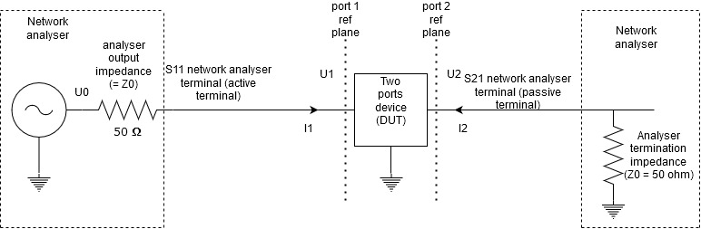
Notice that the analyzer impedance seen from the S21 ref plane is 50 ohm at low frequencies, but also at high frequencies because the characteristic impedance of the cable is just 50 ohm. That means that this diagram is valid at all frequencies.- This being said, according to the article cited in the question, with
- $$a_i = \frac{U_i + Z_0I_i}{2\sqrt{Z_0}}\ \ \text{and} \ \
- b_i = \frac{U_i - Z_0I_i}{2\sqrt{Z_0}}, $$
- we have, for $(i, j) = (1,1)$ and $(i, j) = (2, 1)$,
- $$ S_{ij} = \frac{b_i}{a_j}.$$
- The rest consists in computing $U_i$ and $I_i$ with complex analysis, using the usual electrical circuit laws.
- Let us apply that to our problem:
- 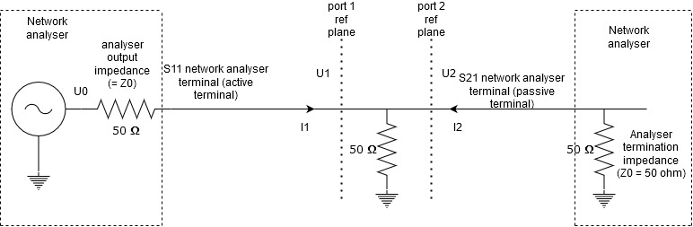
- We have
- $$I_1 = U_1 / (50\Omega || 50\Omega) = U_1/25;$$
- $$I_2 = -U_2/50 = -U_1/50;$$
- Omitting the $1/2\sqrt{Z_0}$ factor that vanishes in the fractions below, we then have
- $$a_1 = U_1+ \frac{50}{25}U_1 = 3U_1, \ \ b_1 = U_1- \frac{50}{25}U_1= -U_1,\ \ b_2 = U_2 +\frac{50}{50}U_1 = U_1+U_1 = 2U_1.$$
- We deduce
- $$S_{11} = \frac{b_1}{a_1} = -\frac{1}{3} = -0.33\ldots \ \ \text{and}\ \ S_{21} = \frac{b_2}{a_1} = \frac{2}{3} = 0.66\ldots$$
- BINGO!!!
- Eureka! thanks to the article cited in the question, I've finally understood the matter.
- I will describe here the general procedure for computing the network parameters of a grounded two port device (DUT), without entering into the intuition behind the math. The generalization to more ports is easy.
- Let me call "active terminal" the terminal of the analyzer that sends the stimulus, that is, the S11 terminal. Similarly, let me call "passive terminal" the S21 terminal of the analyzer.
- The first point to understand is, as vaguely suggested by the cited article, that the signal exiting from the active terminal of the network analyzer has a given output impedance. I believe that in general, most analyzers are built in such a way that this impedance is equal to the characteristic impedance of the usual coaxial cables, that is, 50 ohm. This will be assumed here for the sake of completeness, but be aware that this impedance plays no role in the computations below.
- At the other end, the passive terminal entering into the analyzer is terminated by a resistance equal to the characteristic impedance of the cables, that is, 50 ohm again.
- Thus, we have the following diagram:
- 
- Notice that the analyzer termination impedance seen from the S21 ref plane is 50 ohm at low frequencies, but also at high frequencies because the characteristic impedance of the cable is just 50 ohm. That means that this diagram is valid at all frequencies.
- This being said, according to the article cited in the question, with
- $$a_i = \frac{U_i + Z_0I_i}{2\sqrt{Z_0}}\ \ \text{and} \ \
- b_i = \frac{U_i - Z_0I_i}{2\sqrt{Z_0}}, $$
- we have, for $(i, j) = (1,1)$ and $(i, j) = (2, 1)$,
- $$ S_{ij} = \frac{b_i}{a_j}.$$
- The rest consists in computing $U_i$ and $I_i$ with complex analysis, using the usual electrical circuit laws.
- Let us apply that to our problem:
- 
- We have
- $$I_1 = U_1 / (50\Omega || 50\Omega) = U_1/25;$$
- $$I_2 = -U_2/50 = -U_1/50;$$
- Omitting the $1/2\sqrt{Z_0}$ factor that vanishes in the fractions below, we then have
- $$a_1 = U_1+ \frac{50}{25}U_1 = 3U_1, \ \ b_1 = U_1- \frac{50}{25}U_1= -U_1,\ \ b_2 = U_2 +\frac{50}{50}U_1 = U_1+U_1 = 2U_1.$$
- We deduce
- $$S_{11} = \frac{b_1}{a_1} = -\frac{1}{3} = -0.33\ldots \ \ \text{and}\ \ S_{21} = \frac{b_2}{a_1} = \frac{2}{3} = 0.66\ldots$$
- BINGO!!!
#5: Post edited
by
coquelicot
·
2020-11-15T15:13:41Z (over 4 years ago)
- Eureka! thanks to the article cited in the question, I've finally understood the matter.
- I will describe here the general procedure for computing the network parameters of a grounded two port device (DUT), without entering into the intuition behind the math. The generalization to more ports is easy.
- Let me call "active terminal" the terminal of the analyzer that sends the stimulus, that is, the S11 terminal. Similarly, let me call "passive terminal" the S21 terminal of the analyzer.
The first point to understand is, as vaguely suggested by the cited article, that the signal exiting from the active terminal of the network analyzer has a given output impedance. I believe that in general, most analyzers are built in such a way that this impedance is equal to the characteristic impedance of the usual coaxial cables, that is, 50 ohm. This will be assumed here. At the other end, the passive terminal entering into the analyzer is terminated by a resistance equal to the characteristic impedance of the cables, that is, 50 ohm again.- Thus, we have the following diagram:
- 
- Notice that the analyzer impedance seen from the S21 ref plane is 50 ohm at low frequencies, but also at high frequencies because the characteristic impedance of the cable is just 50 ohm. That means that this diagram is valid at all frequencies.
- This being said, according to the article cited in the question, with
- $$a_i = \frac{U_i + Z_0I_i}{2\sqrt{Z_0}}\ \ \text{and} \ \
- b_i = \frac{U_i - Z_0I_i}{2\sqrt{Z_0}}, $$
- we have, for $(i, j) = (1,1)$ and $(i, j) = (2, 1)$,
- $$ S_{ij} = \frac{b_i}{a_j}.$$
- The rest consists in computing $U_i$ and $I_i$ with complex analysis, using the usual electrical circuit laws.
- Let us apply that to our problem:
- 
- We have
- $$I_1 = U_1 / (50\Omega || 50\Omega) = U_1/25;$$
- $$I_2 = -U_2/50 = -U_1/50;$$
- Omitting the $1/2\sqrt{Z_0}$ factor that vanishes in the fractions below, we then have
- $$a_1 = U_1+ \frac{50}{25}U_1 = 3U_1, \ \ b_1 = U_1- \frac{50}{25}U_1= -U_1,\ \ b_2 = U_2 +\frac{50}{50}U_1 = U_1+U_1 = 2U_1.$$
- We deduce
- $$S_{11} = \frac{b_1}{a_1} = -\frac{1}{3} = -0.33\ldots \ \ \text{and}\ \ S_{21} = \frac{b_2}{a_1} = \frac{2}{3} = 0.66\ldots$$
- BINGO!!!
- Eureka! thanks to the article cited in the question, I've finally understood the matter.
- I will describe here the general procedure for computing the network parameters of a grounded two port device (DUT), without entering into the intuition behind the math. The generalization to more ports is easy.
- Let me call "active terminal" the terminal of the analyzer that sends the stimulus, that is, the S11 terminal. Similarly, let me call "passive terminal" the S21 terminal of the analyzer.
- The first point to understand is, as vaguely suggested by the cited article, that the signal exiting from the active terminal of the network analyzer has a given output impedance. I believe that in general, most analyzers are built in such a way that this impedance is equal to the characteristic impedance of the usual coaxial cables, that is, 50 ohm. This will be assumed here for the sake of completeness, but be aware that this impedance plays no role in the computations below.
- At the other end, the passive terminal entering into the analyzer is terminated by a resistance equal to the characteristic impedance of the cables, that is, 50 ohm again.
- Thus, we have the following diagram:
- 
- Notice that the analyzer impedance seen from the S21 ref plane is 50 ohm at low frequencies, but also at high frequencies because the characteristic impedance of the cable is just 50 ohm. That means that this diagram is valid at all frequencies.
- This being said, according to the article cited in the question, with
- $$a_i = \frac{U_i + Z_0I_i}{2\sqrt{Z_0}}\ \ \text{and} \ \
- b_i = \frac{U_i - Z_0I_i}{2\sqrt{Z_0}}, $$
- we have, for $(i, j) = (1,1)$ and $(i, j) = (2, 1)$,
- $$ S_{ij} = \frac{b_i}{a_j}.$$
- The rest consists in computing $U_i$ and $I_i$ with complex analysis, using the usual electrical circuit laws.
- Let us apply that to our problem:
- 
- We have
- $$I_1 = U_1 / (50\Omega || 50\Omega) = U_1/25;$$
- $$I_2 = -U_2/50 = -U_1/50;$$
- Omitting the $1/2\sqrt{Z_0}$ factor that vanishes in the fractions below, we then have
- $$a_1 = U_1+ \frac{50}{25}U_1 = 3U_1, \ \ b_1 = U_1- \frac{50}{25}U_1= -U_1,\ \ b_2 = U_2 +\frac{50}{50}U_1 = U_1+U_1 = 2U_1.$$
- We deduce
- $$S_{11} = \frac{b_1}{a_1} = -\frac{1}{3} = -0.33\ldots \ \ \text{and}\ \ S_{21} = \frac{b_2}{a_1} = \frac{2}{3} = 0.66\ldots$$
- BINGO!!!
#4: Post edited
by
coquelicot
·
2020-11-15T13:13:19Z (over 4 years ago)
- Eureka! thanks to the article cited in the question, I've finally understood the matter.
- I will describe here the general procedure for computing the network parameters of a grounded two port device (DUT), without entering into the intuition behind the math. The generalization to more ports is easy.
- Let me call "active terminal" the terminal of the analyzer that sends the stimulus, that is, the S11 terminal. Similarly, let me call "passive terminal" the S21 terminal of the analyzer.
- The first point to understand is, as vaguely suggested by the cited article, that the signal exiting from the active terminal of the network analyzer has a given output impedance. I believe that in general, most analyzers are built in such a way that this impedance is equal to the characteristic impedance of the usual coaxial cables, that is, 50 ohm. This will be assumed here. At the other end, the passive terminal entering into the analyzer is terminated by a resistance equal to the characteristic impedance of the cables, that is, 50 ohm again.
- Thus, we have the following diagram:
- 
- Notice that the analyzer impedance seen from the S21 ref plane is 50 ohm at low frequencies, but also at high frequencies because the characteristic impedance of the cable is just 50 ohm. That means that this diagram is valid at all frequencies.
- This being said, according to the article cited in the question, with
- $$a_i = \frac{U_i + Z_0I_i}{2\sqrt{Z_0}}\ \ \text{and} \ \
- b_i = \frac{U_i - Z_0I_i}{2\sqrt{Z_0}}, $$
- we have, for $(i, j) = (1,1)$ and $(i, j) = (2, 1)$,
- $$ S_{ij} = \frac{b_i}{a_j}.$$
- The rest consists in computing $U_i$ and $I_i$ with complex analysis, using the usual electrical circuit laws.
- Let us apply that to our problem:
- 
- We have
- $$I_1 = U_1 / (50\Omega || 50\Omega) = U_1/25;$$
- $$I_2 = -U_2/50 = -U_1/50;$$
Omitting the $1/2\sqrt(Z_0)$ factor that vanishes in the fractions below, we then have- $$a_1 = U_1+ \frac{50}{25}U_1 = 3U_1, \ \ b_1 = U_1- \frac{50}{25}U_1= -U_1,\ \ b_2 = U_2 +\frac{50}{50}U_1 = U_1+U_1 = 2U_1.$$
- We deduce
- $$S_{11} = \frac{b_1}{a_1} = -\frac{1}{3} = -0.33\ldots \ \ \text{and}\ \ S_{21} = \frac{b_2}{a_1} = \frac{2}{3} = 0.66\ldots$$
- BINGO!!!
- Eureka! thanks to the article cited in the question, I've finally understood the matter.
- I will describe here the general procedure for computing the network parameters of a grounded two port device (DUT), without entering into the intuition behind the math. The generalization to more ports is easy.
- Let me call "active terminal" the terminal of the analyzer that sends the stimulus, that is, the S11 terminal. Similarly, let me call "passive terminal" the S21 terminal of the analyzer.
- The first point to understand is, as vaguely suggested by the cited article, that the signal exiting from the active terminal of the network analyzer has a given output impedance. I believe that in general, most analyzers are built in such a way that this impedance is equal to the characteristic impedance of the usual coaxial cables, that is, 50 ohm. This will be assumed here. At the other end, the passive terminal entering into the analyzer is terminated by a resistance equal to the characteristic impedance of the cables, that is, 50 ohm again.
- Thus, we have the following diagram:
- 
- Notice that the analyzer impedance seen from the S21 ref plane is 50 ohm at low frequencies, but also at high frequencies because the characteristic impedance of the cable is just 50 ohm. That means that this diagram is valid at all frequencies.
- This being said, according to the article cited in the question, with
- $$a_i = \frac{U_i + Z_0I_i}{2\sqrt{Z_0}}\ \ \text{and} \ \
- b_i = \frac{U_i - Z_0I_i}{2\sqrt{Z_0}}, $$
- we have, for $(i, j) = (1,1)$ and $(i, j) = (2, 1)$,
- $$ S_{ij} = \frac{b_i}{a_j}.$$
- The rest consists in computing $U_i$ and $I_i$ with complex analysis, using the usual electrical circuit laws.
- Let us apply that to our problem:
- 
- We have
- $$I_1 = U_1 / (50\Omega || 50\Omega) = U_1/25;$$
- $$I_2 = -U_2/50 = -U_1/50;$$
- Omitting the $1/2\sqrt{Z_0}$ factor that vanishes in the fractions below, we then have
- $$a_1 = U_1+ \frac{50}{25}U_1 = 3U_1, \ \ b_1 = U_1- \frac{50}{25}U_1= -U_1,\ \ b_2 = U_2 +\frac{50}{50}U_1 = U_1+U_1 = 2U_1.$$
- We deduce
- $$S_{11} = \frac{b_1}{a_1} = -\frac{1}{3} = -0.33\ldots \ \ \text{and}\ \ S_{21} = \frac{b_2}{a_1} = \frac{2}{3} = 0.66\ldots$$
- BINGO!!!
#3: Post edited
by
coquelicot
·
2020-11-15T13:12:47Z (over 4 years ago)
- Eureka! thanks to the article cited in the question, I've finally understood the matter.
- I will describe here the general procedure for computing the network parameters of a grounded two port device (DUT), without entering into the intuition behind the math. The generalization to more ports is easy.
- Let me call "active terminal" the terminal of the analyzer that sends the stimulus, that is, the S11 terminal. Similarly, let me call "passive terminal" the S21 terminal of the analyzer.
- The first point to understand is, as vaguely suggested by the cited article, that the signal exiting from the active terminal of the network analyzer has a given output impedance. I believe that in general, most analyzers are built in such a way that this impedance is equal to the characteristic impedance of the usual coaxial cables, that is, 50 ohm. This will be assumed here. At the other end, the passive terminal entering into the analyzer is terminated by a resistance equal to the characteristic impedance of the cables, that is, 50 ohm again.
- Thus, we have the following diagram:
- 
- Notice that the analyzer impedance seen from the S21 ref plane is 50 ohm at low frequencies, but also at high frequencies because the characteristic impedance of the cable is just 50 ohm. That means that this diagram is valid at all frequencies.
- This being said, according to the article cited in the question, with
$$a_i = \frac{U_i + Z_0I_i}{\sqrt{Z_0}}\ \ \text{and} \ \b_i = \frac{U_i - Z_0I_i}{\sqrt{Z_0}}, $$- we have, for $(i, j) = (1,1)$ and $(i, j) = (2, 1)$,
- $$ S_{ij} = \frac{b_i}{a_j}.$$
- The rest consists in computing $U_i$ and $I_i$ with complex analysis, using the usual electrical circuit laws.
- Let us apply that to our problem:
- 
- We have
- $$I_1 = U_1 / (50\Omega || 50\Omega) = U_1/25;$$
- $$I_2 = -U_2/50 = -U_1/50;$$
Omitting the $1/\sqrt(Z_0)$ factor that vanishes in the fractions below, we then have- $$a_1 = U_1+ \frac{50}{25}U_1 = 3U_1, \ \ b_1 = U_1- \frac{50}{25}U_1= -U_1,\ \ b_2 = U_2 +\frac{50}{50}U_1 = U_1+U_1 = 2U_1.$$
- We deduce
- $$S_{11} = \frac{b_1}{a_1} = -\frac{1}{3} = -0.33\ldots \ \ \text{and}\ \ S_{21} = \frac{b_2}{a_1} = \frac{2}{3} = 0.66\ldots$$
- BINGO!!!
- Eureka! thanks to the article cited in the question, I've finally understood the matter.
- I will describe here the general procedure for computing the network parameters of a grounded two port device (DUT), without entering into the intuition behind the math. The generalization to more ports is easy.
- Let me call "active terminal" the terminal of the analyzer that sends the stimulus, that is, the S11 terminal. Similarly, let me call "passive terminal" the S21 terminal of the analyzer.
- The first point to understand is, as vaguely suggested by the cited article, that the signal exiting from the active terminal of the network analyzer has a given output impedance. I believe that in general, most analyzers are built in such a way that this impedance is equal to the characteristic impedance of the usual coaxial cables, that is, 50 ohm. This will be assumed here. At the other end, the passive terminal entering into the analyzer is terminated by a resistance equal to the characteristic impedance of the cables, that is, 50 ohm again.
- Thus, we have the following diagram:
- 
- Notice that the analyzer impedance seen from the S21 ref plane is 50 ohm at low frequencies, but also at high frequencies because the characteristic impedance of the cable is just 50 ohm. That means that this diagram is valid at all frequencies.
- This being said, according to the article cited in the question, with
- $$a_i = \frac{U_i + Z_0I_i}{2\sqrt{Z_0}}\ \ \text{and} \ \
- b_i = \frac{U_i - Z_0I_i}{2\sqrt{Z_0}}, $$
- we have, for $(i, j) = (1,1)$ and $(i, j) = (2, 1)$,
- $$ S_{ij} = \frac{b_i}{a_j}.$$
- The rest consists in computing $U_i$ and $I_i$ with complex analysis, using the usual electrical circuit laws.
- Let us apply that to our problem:
- 
- We have
- $$I_1 = U_1 / (50\Omega || 50\Omega) = U_1/25;$$
- $$I_2 = -U_2/50 = -U_1/50;$$
- Omitting the $1/2\sqrt(Z_0)$ factor that vanishes in the fractions below, we then have
- $$a_1 = U_1+ \frac{50}{25}U_1 = 3U_1, \ \ b_1 = U_1- \frac{50}{25}U_1= -U_1,\ \ b_2 = U_2 +\frac{50}{50}U_1 = U_1+U_1 = 2U_1.$$
- We deduce
- $$S_{11} = \frac{b_1}{a_1} = -\frac{1}{3} = -0.33\ldots \ \ \text{and}\ \ S_{21} = \frac{b_2}{a_1} = \frac{2}{3} = 0.66\ldots$$
- BINGO!!!
#2: Post edited
by
coquelicot
·
2020-11-15T12:54:18Z (over 4 years ago)
- Eureka! thanks to the article cited in the question, I've finally understood the matter.
- I will describe here the general procedure for computing the network parameters of a grounded two port device (DUT), without entering into the intuition behind the math. The generalization to more ports is easy.
- Let me call "active terminal" the terminal of the analyzer that sends the stimulus, that is, the S11 terminal. Similarly, let me call "passive terminal" the S21 terminal of the analyzer.
- The first point to understand is, as vaguely suggested by the cited article, that the signal exiting from the active terminal of the network analyzer has a given output impedance. I believe that in general, most analyzers are built in such a way that this impedance is equal to the characteristic impedance of the usual coaxial cables, that is, 50 ohm. This will be assumed here. At the other end, the passive terminal entering into the analyzer is terminated by a resistance equal to the characteristic impedance of the cables, that is, 50 ohm again.
- Thus, we have the following diagram:
- 
- Notice that the analyzer impedance seen from the S21 ref plane is 50 ohm at low frequencies, but also at high frequencies because the characteristic impedance of the cable is just 50 ohm. That means that this diagram is valid at all frequencies.
- This being said, according to the article cited in the question, with
- $$a_i = \frac{U_i + Z_0I_i}{\sqrt{Z_0}}\ \ \text{and} \ \
- b_i = \frac{U_i - Z_0I_i}{\sqrt{Z_0}}, $$
- we have, for $(i, j) = (1,1)$ and $(i, j) = (2, 1)$,
- $$ S_{ij} = \frac{b_i}{a_j}.$$
- The rest consists in computing $U_i$ and $I_i$ with complex analysis, using the usual electrical circuit laws.
- Let us apply that to our problem:
- 
- We have
- $$I_1 = U_1 / (50\Omega || 50\Omega) = U_1/25;$$
- $$I_2 = -U_2/50 = -U_1/50;$$
- Omitting the $1/\sqrt(Z_0)$ factor that vanishes in the fractions below, we then have
- $$a_1 = U_1+ \frac{50}{25}U_1 = 3U_1, \ \ b_1 = U_1- \frac{50}{25}U_1= -U_1,\ \ b_2 = U_2 +\frac{50}{50}U_1 = U_1+U_1 = 2U_1.$$
- We deduce
$$S_{11} = \frac{b_1}{a_1} = -\frac{1}{3} = -0.33 \ \ \text{and}\ \ S_{21} = \frac{b_2}{a_1} = \frac{2}{3} = 0.66.$$- BINGO!!!
- Eureka! thanks to the article cited in the question, I've finally understood the matter.
- I will describe here the general procedure for computing the network parameters of a grounded two port device (DUT), without entering into the intuition behind the math. The generalization to more ports is easy.
- Let me call "active terminal" the terminal of the analyzer that sends the stimulus, that is, the S11 terminal. Similarly, let me call "passive terminal" the S21 terminal of the analyzer.
- The first point to understand is, as vaguely suggested by the cited article, that the signal exiting from the active terminal of the network analyzer has a given output impedance. I believe that in general, most analyzers are built in such a way that this impedance is equal to the characteristic impedance of the usual coaxial cables, that is, 50 ohm. This will be assumed here. At the other end, the passive terminal entering into the analyzer is terminated by a resistance equal to the characteristic impedance of the cables, that is, 50 ohm again.
- Thus, we have the following diagram:
- 
- Notice that the analyzer impedance seen from the S21 ref plane is 50 ohm at low frequencies, but also at high frequencies because the characteristic impedance of the cable is just 50 ohm. That means that this diagram is valid at all frequencies.
- This being said, according to the article cited in the question, with
- $$a_i = \frac{U_i + Z_0I_i}{\sqrt{Z_0}}\ \ \text{and} \ \
- b_i = \frac{U_i - Z_0I_i}{\sqrt{Z_0}}, $$
- we have, for $(i, j) = (1,1)$ and $(i, j) = (2, 1)$,
- $$ S_{ij} = \frac{b_i}{a_j}.$$
- The rest consists in computing $U_i$ and $I_i$ with complex analysis, using the usual electrical circuit laws.
- Let us apply that to our problem:
- 
- We have
- $$I_1 = U_1 / (50\Omega || 50\Omega) = U_1/25;$$
- $$I_2 = -U_2/50 = -U_1/50;$$
- Omitting the $1/\sqrt(Z_0)$ factor that vanishes in the fractions below, we then have
- $$a_1 = U_1+ \frac{50}{25}U_1 = 3U_1, \ \ b_1 = U_1- \frac{50}{25}U_1= -U_1,\ \ b_2 = U_2 +\frac{50}{50}U_1 = U_1+U_1 = 2U_1.$$
- We deduce
- $$S_{11} = \frac{b_1}{a_1} = -\frac{1}{3} = -0.33\ldots \ \ \text{and}\ \ S_{21} = \frac{b_2}{a_1} = \frac{2}{3} = 0.66\ldots$$
- BINGO!!!
#1: Initial revision
by
coquelicot
·
2020-11-15T11:36:19Z (over 4 years ago)
Eureka! thanks to the article cited in the question, I've finally understood the matter.
I will describe here the general procedure for computing the network parameters of a grounded two port device (DUT), without entering into the intuition behind the math. The generalization to more ports is easy.
Let me call "active terminal" the terminal of the analyzer that sends the stimulus, that is, the S11 terminal. Similarly, let me call "passive terminal" the S21 terminal of the analyzer.
The first point to understand is, as vaguely suggested by the cited article, that the signal exiting from the active terminal of the network analyzer has a given output impedance. I believe that in general, most analyzers are built in such a way that this impedance is equal to the characteristic impedance of the usual coaxial cables, that is, 50 ohm. This will be assumed here. At the other end, the passive terminal entering into the analyzer is terminated by a resistance equal to the characteristic impedance of the cables, that is, 50 ohm again.
Thus, we have the following diagram:

Notice that the analyzer impedance seen from the S21 ref plane is 50 ohm at low frequencies, but also at high frequencies because the characteristic impedance of the cable is just 50 ohm. That means that this diagram is valid at all frequencies.
This being said, according to the article cited in the question, with
$$a_i = \frac{U_i + Z_0I_i}{\sqrt{Z_0}}\ \ \text{and} \ \
b_i = \frac{U_i - Z_0I_i}{\sqrt{Z_0}}, $$
we have, for $(i, j) = (1,1)$ and $(i, j) = (2, 1)$,
$$ S_{ij} = \frac{b_i}{a_j}.$$
The rest consists in computing $U_i$ and $I_i$ with complex analysis, using the usual electrical circuit laws.
Let us apply that to our problem:

We have
$$I_1 = U_1 / (50\Omega || 50\Omega) = U_1/25;$$
$$I_2 = -U_2/50 = -U_1/50;$$
Omitting the $1/\sqrt(Z_0)$ factor that vanishes in the fractions below, we then have
$$a_1 = U_1+ \frac{50}{25}U_1 = 3U_1, \ \ b_1 = U_1- \frac{50}{25}U_1= -U_1,\ \ b_2 = U_2 +\frac{50}{50}U_1 = U_1+U_1 = 2U_1.$$
We deduce
$$S_{11} = \frac{b_1}{a_1} = -\frac{1}{3} = -0.33 \ \ \text{and}\ \ S_{21} = \frac{b_2}{a_1} = \frac{2}{3} = 0.66.$$
BINGO!!!