Post History
A loss-less coaxial cable has inductance and capacitance and, their associated formulas introduce $\epsilon$ and $\mu$. But, to home-in on the velocity of propagation, the characteristic impedance ...
#15: Post edited
by
 Andy aka
·
2023-12-25T11:59:59Z (over 1 year ago)
Andy aka
·
2023-12-25T11:59:59Z (over 1 year ago)
- A **loss-less** coaxial cable has inductance and capacitance and, their associated formulas introduce \$\epsilon\$ and \$\mu\$. But, to home-in on the velocity of propagation, the characteristic impedance must also be determined. We can avoid the complexity of the telegrapher's equations by looking at a short piece of **loss-less** cable in the frequency domain: -
- <sub>$$$$</sub>
- 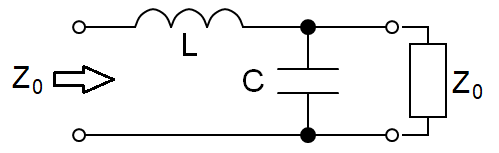
- $$Z_0\hspace{1cm} = \hspace{1cm}sL + \dfrac{\frac{1}{sC}\cdot Z_0}{\frac{1}{sC} + Z_0}\hspace{1cm}=\hspace{1cm} sL + \dfrac{Z_0}{1 + sCZ_0}$$
- $$Z_0 + sCZ_0^2\hspace{1cm} =\hspace{1cm} sL + s^2LCZ_0 + Z_0$$
- $$sCZ_0^2 \hspace{1cm}=\hspace{1cm} sL + s^2LCZ_0$$
- <sub>$$$$</sub>
- When s, L and C are small, we can ignore the \$s^2LCZ_0\$ term, hence: -
- $$sCZ_0^2 = sL$$
- And, \$\hspace{7cm}Z_0 = \sqrt{\dfrac{L}{C}}\hspace{1cm}\$ (a well known formula).
- <sub>$$$$</sub>
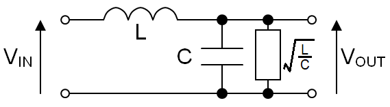
- Having \$Z_0\$, we can analyse the circuit's transfer function. This allows us to find the output phase lag and, with a little more manipulation, the time delay for 1 metre of cable: -
- 
- <sub>$$$$</sub>
- A general bode plot using lumped-values for L and C (per metre) is of interest: -
- 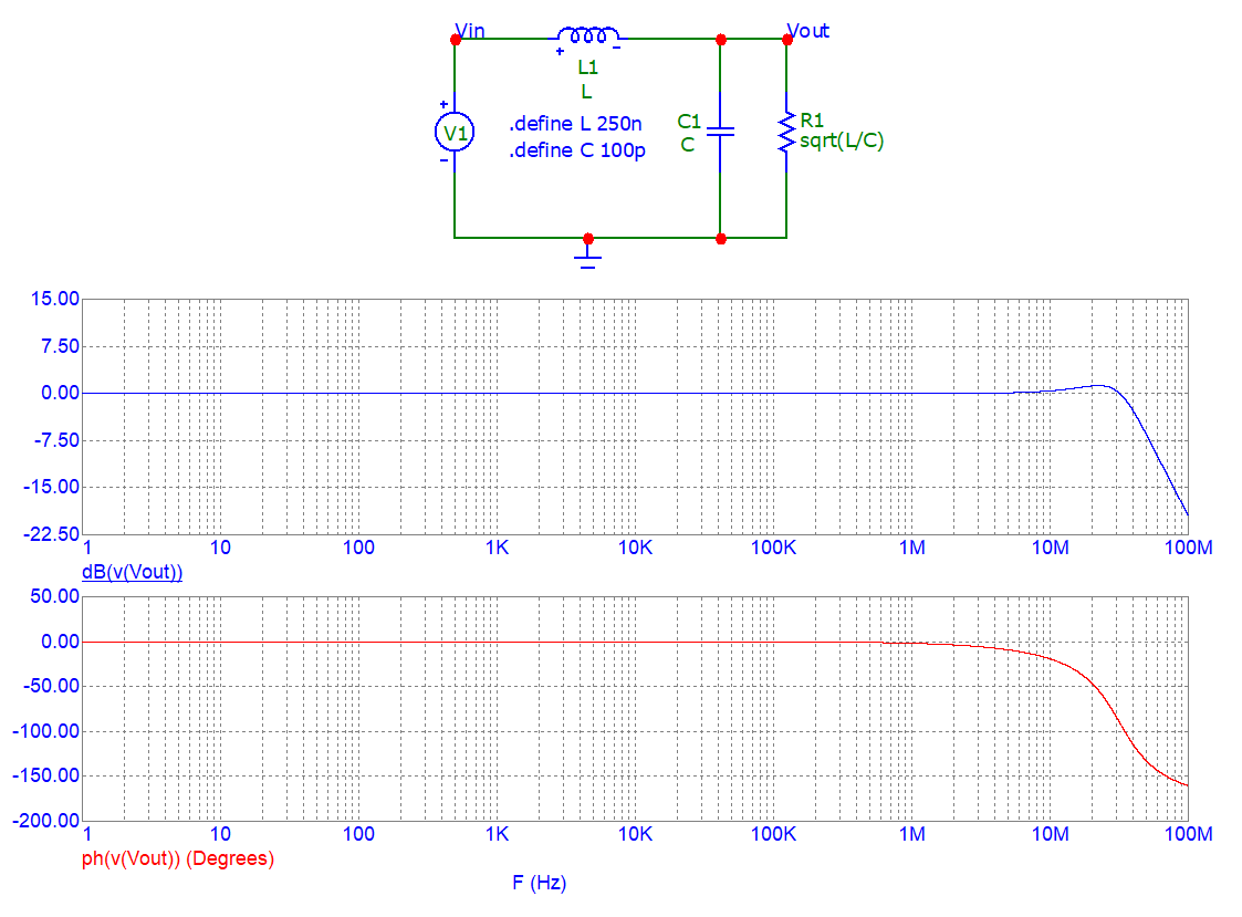
- Here's a close-up of the phase response plotted linearly against frequency up to 1 MHz: -
- 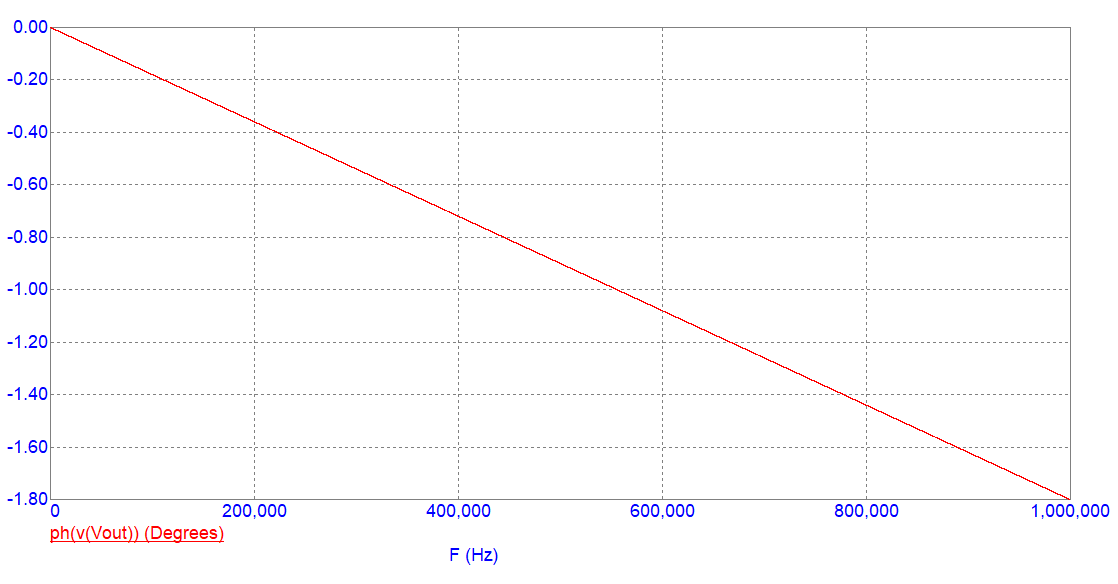
- - At 1 MHz, the output phase lag is 1.8°
- - As a fraction of the period (1 μs) it's 0.005 hence, it's a time lag of 5 ns.
- - At 100 kHz, the phase lag is 0.18° but, it's still a time lag of 5 ns
Given that I've modelled 1 metre lengths of capacitance and inductance, the equivalent velocity of propagation has to be 200 million metres per second. It's just the inverse of the time lag.- <sub>$$$$</sub>
- A simulator is great as a demonstrator but, a phase angle formula is needed so that we know what the dependencies are. It's a simple 2nd order low pass filter and, if you went through the derivation (omitted to keep the answer shorter) you find this: -
- $$\text{Phase lag} = \arctan\left(\dfrac{2\zeta\dfrac{\omega}{\omega_n}}{1 - \dfrac{\omega^2}{\omega_n^2}}\right)$$
- Because we are making \$\omega\$ a lot smaller than \$\omega_n\$ we can simplify: -
- - The arctan of a small number **is** the small number because
- $$\arctan(x) = x - \frac{x^3}{3} + \frac{x^5}{5} - ...$$
- - The denominator equals 1
- $$\text{Phase lag} = {2\zeta\dfrac{\omega}{\omega_n}}$$
- But, we can also determine \$\zeta\$ for the circuit. [Wikipedia RLC circuits](https://en.wikibooks.org/wiki/Circuit_Theory/RLC_Circuits#Damping_Factor) shows it is this: -
- 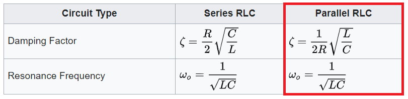
- And, because we know that R is \$Z_0\$ \$\left(\sqrt{\frac{L}{C}}\right)\$, \$\zeta\$ must equal 0.5. The phase lag now becomes: -
- $$\text{Phase lag} = {\dfrac{\omega}{\omega_n}} = \omega\sqrt{LC}$$
- <sub>Anyone studying telegrapher's equations will recognize this as the imaginary part of the propagation constant.$$$$</sub>
- Dividing the phase lag by \$\omega\$ gives us the time lag: -
- $$\text{Time lag} = \dfrac{1}{\omega_n} = \sqrt{LC}$$
- And, the velocity of propagation is the reciprocal of the time lag (for a 1 metre length of cable): -
- $$\text{Velocity of propagation} = \dfrac{1}{\sqrt{LC}}$$
- Nearly there!
- $$$$
- Right at the start I mentioned coaxial cable and its inductance and capacitance per unit length. The formulas are: -
- $$L = \dfrac{\mu}{2\pi}\ln\left(\dfrac{b}{a}\right)$$
- Taken from [Inductance of a Coaxial Structure](https://eng.libretexts.org/Bookshelves/Electrical_Engineering/Electro-Optics/Book%3A_Electromagnetics_I_(Ellingson)/07%3A_Magnetostatics/7.14%3A_Inductance_of_a_Coaxial_Structure#:~:text=Below%20we%20shall%20find%20the,flux%20to%20the%20source%20current.)
- $$C = \dfrac{2\pi\epsilon}{\ln\left(\dfrac{b}{a}\right)}$$
- Taken from [Capacitance of a coaxial structure](https://eng.libretexts.org/Bookshelves/Electrical_Engineering/Electro-Optics/Book%3A_Electromagnetics_I_(Ellingson)/05%3A_Electrostatics/5.24%3A_Capacitance_of_a_Coaxial_Structure)
- $$$$
- If we multiply L and C we get \$\epsilon\cdot\mu\$ hence,
- $$\text{Velocity of propagation} = \dfrac{1}{\sqrt{\epsilon\cdot\mu}}$$
- A **loss-less** coaxial cable has inductance and capacitance and, their associated formulas introduce \$\epsilon\$ and \$\mu\$. But, to home-in on the velocity of propagation, the characteristic impedance must also be determined. We can avoid the complexity of the telegrapher's equations by looking at a short piece of **loss-less** cable in the frequency domain: -
- <sub>$$$$</sub>
- 
- $$Z_0\hspace{1cm} = \hspace{1cm}sL + \dfrac{\frac{1}{sC}\cdot Z_0}{\frac{1}{sC} + Z_0}\hspace{1cm}=\hspace{1cm} sL + \dfrac{Z_0}{1 + sCZ_0}$$
- $$Z_0 + sCZ_0^2\hspace{1cm} =\hspace{1cm} sL + s^2LCZ_0 + Z_0$$
- $$sCZ_0^2 \hspace{1cm}=\hspace{1cm} sL + s^2LCZ_0$$
- <sub>$$$$</sub>
- When s, L and C are small, we can ignore the \$s^2LCZ_0\$ term, hence: -
- $$sCZ_0^2 = sL$$
- And, \$\hspace{7cm}Z_0 = \sqrt{\dfrac{L}{C}}\hspace{1cm}\$ (a well known formula).
- <sub>$$$$</sub>
- Having \$Z_0\$, we can analyse the circuit's transfer function. This allows us to find the output phase lag and, with a little more manipulation, the time delay for 1 metre of cable: -
- 
- <sub>$$$$</sub>
- A general bode plot using lumped-values for L and C (per metre) is of interest: -
- 
- Here's a close-up of the phase response plotted linearly against frequency up to 1 MHz: -
- 
- - At 1 MHz, the output phase lag is 1.8°
- - As a fraction of the period (1 μs) it's 0.005 hence, it's a time lag of 5 ns.
- - At 100 kHz, the phase lag is 0.18° but, it's still a time lag of 5 ns
- Because 1 metre lengths of capacitance and inductance are modelled, the equivalent velocity of propagation is 200 million metres per second (the inverse of the time lag).
- <sub>$$$$</sub>
- A simulator is great as a demonstrator but, a phase angle formula is needed so that we know what the dependencies are. It's a simple 2nd order low pass filter and, if you went through the derivation (omitted to keep the answer shorter) you find this: -
- $$\text{Phase lag} = \arctan\left(\dfrac{2\zeta\dfrac{\omega}{\omega_n}}{1 - \dfrac{\omega^2}{\omega_n^2}}\right)$$
- Because we are making \$\omega\$ a lot smaller than \$\omega_n\$ we can simplify: -
- - The arctan of a small number **is** the small number because
- $$\arctan(x) = x - \frac{x^3}{3} + \frac{x^5}{5} - ...$$
- - The denominator equals 1
- $$\text{Phase lag} = {2\zeta\dfrac{\omega}{\omega_n}}$$
- But, we can also determine \$\zeta\$ for the circuit. [Wikipedia RLC circuits](https://en.wikibooks.org/wiki/Circuit_Theory/RLC_Circuits#Damping_Factor) shows it is this: -
- 
- And, because we know that R is \$Z_0\$ \$\left(\sqrt{\frac{L}{C}}\right)\$, \$\zeta\$ must equal 0.5. The phase lag now becomes: -
- $$\text{Phase lag} = {\dfrac{\omega}{\omega_n}} = \omega\sqrt{LC}$$
- <sub>Anyone studying telegrapher's equations will recognize this as the imaginary part of the propagation constant.$$$$</sub>
- Dividing the phase lag by \$\omega\$ gives us the time lag: -
- $$\text{Time lag} = \dfrac{1}{\omega_n} = \sqrt{LC}$$
- And, the velocity of propagation is the reciprocal of the time lag (for a 1 metre length of cable): -
- $$\text{Velocity of propagation} = \dfrac{1}{\sqrt{LC}}$$
- Nearly there!
- $$$$
- Right at the start I mentioned coaxial cable and its inductance and capacitance per unit length. The formulas are: -
- $$L = \dfrac{\mu}{2\pi}\ln\left(\dfrac{b}{a}\right)$$
- Taken from [Inductance of a Coaxial Structure](https://eng.libretexts.org/Bookshelves/Electrical_Engineering/Electro-Optics/Book%3A_Electromagnetics_I_(Ellingson)/07%3A_Magnetostatics/7.14%3A_Inductance_of_a_Coaxial_Structure#:~:text=Below%20we%20shall%20find%20the,flux%20to%20the%20source%20current.)
- $$C = \dfrac{2\pi\epsilon}{\ln\left(\dfrac{b}{a}\right)}$$
- Taken from [Capacitance of a coaxial structure](https://eng.libretexts.org/Bookshelves/Electrical_Engineering/Electro-Optics/Book%3A_Electromagnetics_I_(Ellingson)/05%3A_Electrostatics/5.24%3A_Capacitance_of_a_Coaxial_Structure)
- $$$$
- If we multiply L and C we get \$\epsilon\cdot\mu\$ hence,
- $$\text{Velocity of propagation} = \dfrac{1}{\sqrt{\epsilon\cdot\mu}}$$
#14: Post edited
by
Andy aka
·
2023-12-25T11:20:54Z (over 1 year ago)
A **loss-less** coaxial cable has inductance and capacitance and, their associated formulas introduce \$\epsilon\$ and \$\mu\$. But, to home-in on the velocity of propagation, the characteristic impedance should also be determined. We can avoid the complexity of using the telegrapher's equations by analysing a short section of loss-less cable in the frequency domain: -- <sub>$$$$</sub>
- 
$$Z_0 = sL + \dfrac{\frac{1}{sC}\cdot Z_0}{\frac{1}{sC} + Z_0}$$$$Z_0 = sL + \dfrac{Z_0}{1 + sCZ_0}$$$$Z_0 + sCZ_0^2 = sL + s^2LCZ_0 + Z_0$$$$sCZ_0^2 = sL + s^2LCZ_0$$$$$$When s, L and C are small values we can ignore the \$s^2LCZ_0\$ term, hence: -- $$sCZ_0^2 = sL$$
- And, \$\hspace{7cm}Z_0 = \sqrt{\dfrac{L}{C}}\hspace{1cm}\$ (a well known formula).
- <sub>$$$$</sub>
- Having \$Z_0\$, we can analyse the circuit's transfer function. This allows us to find the output phase lag and, with a little more manipulation, the time delay for 1 metre of cable: -
- 
Of particular interest is the phase lag at low to medium frequencies because of its equivalence to time delay (when loaded with the correct value for \$Z_0\$).$$$$A bode plot using lumped-values for L and C (per metre) is revealing: -- 
And, here's a close-up of the phase response plotted linearly against frequency up to 1 MHz: -- 
- - At 1 MHz, the output phase lag is 1.8°
- - As a fraction of the period (1 μs) it's 0.005 hence, it's a time lag of 5 ns.
- - At 100 kHz, the phase lag is 0.18° but, it's still a time lag of 5 ns
- Given that I've modelled 1 metre lengths of capacitance and inductance, the equivalent velocity of propagation has to be 200 million metres per second. It's just the inverse of the time lag.
- <sub>$$$$</sub>
A simulator is great as a demonstrator but, a phase angle formula is needed so that we know what the dependencies are. It's a simple 2nd order low pass filter and, if you went through the derivation (omitted to keep the answer shorter) you find that the phase lag is this: -- $$\text{Phase lag} = \arctan\left(\dfrac{2\zeta\dfrac{\omega}{\omega_n}}{1 - \dfrac{\omega^2}{\omega_n^2}}\right)$$
Then, because we are making \$\omega\$ a lot smaller than \$\omega_n\$ we can make simplifications: -- - The arctan of a small number **is** the small number because
- $$\arctan(x) = x - \frac{x^3}{3} + \frac{x^5}{5} - ...$$
- - The denominator equals 1
- $$\text{Phase lag} = {2\zeta\dfrac{\omega}{\omega_n}}$$
- But, we can also determine \$\zeta\$ for the circuit. [Wikipedia RLC circuits](https://en.wikibooks.org/wiki/Circuit_Theory/RLC_Circuits#Damping_Factor) shows it is this: -
- 
- And, because we know that R is \$Z_0\$ \$\left(\sqrt{\frac{L}{C}}\right)\$, \$\zeta\$ must equal 0.5. The phase lag now becomes: -
- $$\text{Phase lag} = {\dfrac{\omega}{\omega_n}} = \omega\sqrt{LC}$$
- <sub>Anyone studying telegrapher's equations will recognize this as the imaginary part of the propagation constant.$$$$</sub>
- Dividing the phase lag by \$\omega\$ gives us the time lag: -
- $$\text{Time lag} = \dfrac{1}{\omega_n} = \sqrt{LC}$$
- And, the velocity of propagation is the reciprocal of the time lag (for a 1 metre length of cable): -
- $$\text{Velocity of propagation} = \dfrac{1}{\sqrt{LC}}$$
- Nearly there!
- $$$$
- Right at the start I mentioned coaxial cable and its inductance and capacitance per unit length. The formulas are: -
- $$L = \dfrac{\mu}{2\pi}\ln\left(\dfrac{b}{a}\right)$$
- Taken from [Inductance of a Coaxial Structure](https://eng.libretexts.org/Bookshelves/Electrical_Engineering/Electro-Optics/Book%3A_Electromagnetics_I_(Ellingson)/07%3A_Magnetostatics/7.14%3A_Inductance_of_a_Coaxial_Structure#:~:text=Below%20we%20shall%20find%20the,flux%20to%20the%20source%20current.)
- $$C = \dfrac{2\pi\epsilon}{\ln\left(\dfrac{b}{a}\right)}$$
- Taken from [Capacitance of a coaxial structure](https://eng.libretexts.org/Bookshelves/Electrical_Engineering/Electro-Optics/Book%3A_Electromagnetics_I_(Ellingson)/05%3A_Electrostatics/5.24%3A_Capacitance_of_a_Coaxial_Structure)
- $$$$
- If we multiply L and C we get \$\epsilon\cdot\mu\$ hence,
- $$\text{Velocity of propagation} = \dfrac{1}{\sqrt{\epsilon\cdot\mu}}$$
- A **loss-less** coaxial cable has inductance and capacitance and, their associated formulas introduce \$\epsilon\$ and \$\mu\$. But, to home-in on the velocity of propagation, the characteristic impedance must also be determined. We can avoid the complexity of the telegrapher's equations by looking at a short piece of **loss-less** cable in the frequency domain: -
- <sub>$$$$</sub>
- 
- $$Z_0\hspace{1cm} = \hspace{1cm}sL + \dfrac{\frac{1}{sC}\cdot Z_0}{\frac{1}{sC} + Z_0}\hspace{1cm}=\hspace{1cm} sL + \dfrac{Z_0}{1 + sCZ_0}$$
- $$Z_0 + sCZ_0^2\hspace{1cm} =\hspace{1cm} sL + s^2LCZ_0 + Z_0$$
- $$sCZ_0^2 \hspace{1cm}=\hspace{1cm} sL + s^2LCZ_0$$
- <sub>$$$$</sub>
- When s, L and C are small, we can ignore the \$s^2LCZ_0\$ term, hence: -
- $$sCZ_0^2 = sL$$
- And, \$\hspace{7cm}Z_0 = \sqrt{\dfrac{L}{C}}\hspace{1cm}\$ (a well known formula).
- <sub>$$$$</sub>
- Having \$Z_0\$, we can analyse the circuit's transfer function. This allows us to find the output phase lag and, with a little more manipulation, the time delay for 1 metre of cable: -
- 
- <sub>$$$$</sub>
- A general bode plot using lumped-values for L and C (per metre) is of interest: -
- 
- Here's a close-up of the phase response plotted linearly against frequency up to 1 MHz: -
- 
- - At 1 MHz, the output phase lag is 1.8°
- - As a fraction of the period (1 μs) it's 0.005 hence, it's a time lag of 5 ns.
- - At 100 kHz, the phase lag is 0.18° but, it's still a time lag of 5 ns
- Given that I've modelled 1 metre lengths of capacitance and inductance, the equivalent velocity of propagation has to be 200 million metres per second. It's just the inverse of the time lag.
- <sub>$$$$</sub>
- A simulator is great as a demonstrator but, a phase angle formula is needed so that we know what the dependencies are. It's a simple 2nd order low pass filter and, if you went through the derivation (omitted to keep the answer shorter) you find this: -
- $$\text{Phase lag} = \arctan\left(\dfrac{2\zeta\dfrac{\omega}{\omega_n}}{1 - \dfrac{\omega^2}{\omega_n^2}}\right)$$
- Because we are making \$\omega\$ a lot smaller than \$\omega_n\$ we can simplify: -
- - The arctan of a small number **is** the small number because
- $$\arctan(x) = x - \frac{x^3}{3} + \frac{x^5}{5} - ...$$
- - The denominator equals 1
- $$\text{Phase lag} = {2\zeta\dfrac{\omega}{\omega_n}}$$
- But, we can also determine \$\zeta\$ for the circuit. [Wikipedia RLC circuits](https://en.wikibooks.org/wiki/Circuit_Theory/RLC_Circuits#Damping_Factor) shows it is this: -
- 
- And, because we know that R is \$Z_0\$ \$\left(\sqrt{\frac{L}{C}}\right)\$, \$\zeta\$ must equal 0.5. The phase lag now becomes: -
- $$\text{Phase lag} = {\dfrac{\omega}{\omega_n}} = \omega\sqrt{LC}$$
- <sub>Anyone studying telegrapher's equations will recognize this as the imaginary part of the propagation constant.$$$$</sub>
- Dividing the phase lag by \$\omega\$ gives us the time lag: -
- $$\text{Time lag} = \dfrac{1}{\omega_n} = \sqrt{LC}$$
- And, the velocity of propagation is the reciprocal of the time lag (for a 1 metre length of cable): -
- $$\text{Velocity of propagation} = \dfrac{1}{\sqrt{LC}}$$
- Nearly there!
- $$$$
- Right at the start I mentioned coaxial cable and its inductance and capacitance per unit length. The formulas are: -
- $$L = \dfrac{\mu}{2\pi}\ln\left(\dfrac{b}{a}\right)$$
- Taken from [Inductance of a Coaxial Structure](https://eng.libretexts.org/Bookshelves/Electrical_Engineering/Electro-Optics/Book%3A_Electromagnetics_I_(Ellingson)/07%3A_Magnetostatics/7.14%3A_Inductance_of_a_Coaxial_Structure#:~:text=Below%20we%20shall%20find%20the,flux%20to%20the%20source%20current.)
- $$C = \dfrac{2\pi\epsilon}{\ln\left(\dfrac{b}{a}\right)}$$
- Taken from [Capacitance of a coaxial structure](https://eng.libretexts.org/Bookshelves/Electrical_Engineering/Electro-Optics/Book%3A_Electromagnetics_I_(Ellingson)/05%3A_Electrostatics/5.24%3A_Capacitance_of_a_Coaxial_Structure)
- $$$$
- If we multiply L and C we get \$\epsilon\cdot\mu\$ hence,
- $$\text{Velocity of propagation} = \dfrac{1}{\sqrt{\epsilon\cdot\mu}}$$
#13: Post edited
by
Andy aka
·
2023-12-24T18:16:33Z (over 1 year ago)
- A **loss-less** coaxial cable has inductance and capacitance and, their associated formulas introduce \$\epsilon\$ and \$\mu\$. But, to home-in on the velocity of propagation, the characteristic impedance should also be determined. We can avoid the complexity of using the telegrapher's equations by analysing a short section of loss-less cable in the frequency domain: -
- <sub>$$$$</sub>
- 
- $$Z_0 = sL + \dfrac{\frac{1}{sC}\cdot Z_0}{\frac{1}{sC} + Z_0}$$
- $$Z_0 = sL + \dfrac{Z_0}{1 + sCZ_0}$$
- $$Z_0 + sCZ_0^2 = sL + s^2LCZ_0 + Z_0$$
- $$sCZ_0^2 = sL + s^2LCZ_0$$
- $$$$
- When s, L and C are small values we can ignore the \$s^2LCZ_0\$ term, hence: -
- $$sCZ_0^2 = sL$$
- And, \$\hspace{7cm}Z_0 = \sqrt{\dfrac{L}{C}}\hspace{1cm}\$ (a well known formula).
$$$$- Having \$Z_0\$, we can analyse the circuit's transfer function. This allows us to find the output phase lag and, with a little more manipulation, the time delay for 1 metre of cable: -
- 
- Of particular interest is the phase lag at low to medium frequencies because of its equivalence to time delay (when loaded with the correct value for \$Z_0\$).
- $$$$
- A bode plot using lumped-values for L and C (per metre) is revealing: -
- 
- And, here's a close-up of the phase response plotted linearly against frequency up to 1 MHz: -
- 
- - At 1 MHz, the output phase lag is 1.8°
- - As a fraction of the period (1 μs) it's 0.005 hence, it's a time lag of 5 ns.
- - At 100 kHz, the phase lag is 0.18° but, it's still a time lag of 5 ns
- Given that I've modelled 1 metre lengths of capacitance and inductance, the equivalent velocity of propagation has to be 200 million metres per second. It's just the inverse of the time lag.
$$$$- A simulator is great as a demonstrator but, a phase angle formula is needed so that we know what the dependencies are. It's a simple 2nd order low pass filter and, if you went through the derivation (omitted to keep the answer shorter) you find that the phase lag is this: -
- $$\text{Phase lag} = \arctan\left(\dfrac{2\zeta\dfrac{\omega}{\omega_n}}{1 - \dfrac{\omega^2}{\omega_n^2}}\right)$$
- Then, because we are making \$\omega\$ a lot smaller than \$\omega_n\$ we can make simplifications: -
- - The arctan of a small number **is** the small number because
- $$\arctan(x) = x - \frac{x^3}{3} + \frac{x^5}{5} - ...$$
- - The denominator equals 1
- $$\text{Phase lag} = {2\zeta\dfrac{\omega}{\omega_n}}$$
- But, we can also determine \$\zeta\$ for the circuit. [Wikipedia RLC circuits](https://en.wikibooks.org/wiki/Circuit_Theory/RLC_Circuits#Damping_Factor) shows it is this: -
- 
- And, because we know that R is \$Z_0\$ \$\left(\sqrt{\frac{L}{C}}\right)\$, \$\zeta\$ must equal 0.5. The phase lag now becomes: -
- $$\text{Phase lag} = {\dfrac{\omega}{\omega_n}} = \omega\sqrt{LC}$$
- <sub>Anyone studying telegrapher's equations will recognize this as the imaginary part of the propagation constant.$$$$</sub>
- Dividing the phase lag by \$\omega\$ gives us the time lag: -
- $$\text{Time lag} = \dfrac{1}{\omega_n} = \sqrt{LC}$$
- And, the velocity of propagation is the reciprocal of the time lag (for a 1 metre length of cable): -
- $$\text{Velocity of propagation} = \dfrac{1}{\sqrt{LC}}$$
- Nearly there!
- $$$$
- Right at the start I mentioned coaxial cable and its inductance and capacitance per unit length. The formulas are: -
- $$L = \dfrac{\mu}{2\pi}\ln\left(\dfrac{b}{a}\right)$$
- Taken from [Inductance of a Coaxial Structure](https://eng.libretexts.org/Bookshelves/Electrical_Engineering/Electro-Optics/Book%3A_Electromagnetics_I_(Ellingson)/07%3A_Magnetostatics/7.14%3A_Inductance_of_a_Coaxial_Structure#:~:text=Below%20we%20shall%20find%20the,flux%20to%20the%20source%20current.)
- $$C = \dfrac{2\pi\epsilon}{\ln\left(\dfrac{b}{a}\right)}$$
- Taken from [Capacitance of a coaxial structure](https://eng.libretexts.org/Bookshelves/Electrical_Engineering/Electro-Optics/Book%3A_Electromagnetics_I_(Ellingson)/05%3A_Electrostatics/5.24%3A_Capacitance_of_a_Coaxial_Structure)
- $$$$
- If we multiply L and C we get \$\epsilon\cdot\mu\$ hence,
- $$\text{Velocity of propagation} = \dfrac{1}{\sqrt{\epsilon\cdot\mu}}$$
- A **loss-less** coaxial cable has inductance and capacitance and, their associated formulas introduce \$\epsilon\$ and \$\mu\$. But, to home-in on the velocity of propagation, the characteristic impedance should also be determined. We can avoid the complexity of using the telegrapher's equations by analysing a short section of loss-less cable in the frequency domain: -
- <sub>$$$$</sub>
- 
- $$Z_0 = sL + \dfrac{\frac{1}{sC}\cdot Z_0}{\frac{1}{sC} + Z_0}$$
- $$Z_0 = sL + \dfrac{Z_0}{1 + sCZ_0}$$
- $$Z_0 + sCZ_0^2 = sL + s^2LCZ_0 + Z_0$$
- $$sCZ_0^2 = sL + s^2LCZ_0$$
- $$$$
- When s, L and C are small values we can ignore the \$s^2LCZ_0\$ term, hence: -
- $$sCZ_0^2 = sL$$
- And, \$\hspace{7cm}Z_0 = \sqrt{\dfrac{L}{C}}\hspace{1cm}\$ (a well known formula).
- <sub>$$$$</sub>
- Having \$Z_0\$, we can analyse the circuit's transfer function. This allows us to find the output phase lag and, with a little more manipulation, the time delay for 1 metre of cable: -
- 
- Of particular interest is the phase lag at low to medium frequencies because of its equivalence to time delay (when loaded with the correct value for \$Z_0\$).
- $$$$
- A bode plot using lumped-values for L and C (per metre) is revealing: -
- 
- And, here's a close-up of the phase response plotted linearly against frequency up to 1 MHz: -
- 
- - At 1 MHz, the output phase lag is 1.8°
- - As a fraction of the period (1 μs) it's 0.005 hence, it's a time lag of 5 ns.
- - At 100 kHz, the phase lag is 0.18° but, it's still a time lag of 5 ns
- Given that I've modelled 1 metre lengths of capacitance and inductance, the equivalent velocity of propagation has to be 200 million metres per second. It's just the inverse of the time lag.
- <sub>$$$$</sub>
- A simulator is great as a demonstrator but, a phase angle formula is needed so that we know what the dependencies are. It's a simple 2nd order low pass filter and, if you went through the derivation (omitted to keep the answer shorter) you find that the phase lag is this: -
- $$\text{Phase lag} = \arctan\left(\dfrac{2\zeta\dfrac{\omega}{\omega_n}}{1 - \dfrac{\omega^2}{\omega_n^2}}\right)$$
- Then, because we are making \$\omega\$ a lot smaller than \$\omega_n\$ we can make simplifications: -
- - The arctan of a small number **is** the small number because
- $$\arctan(x) = x - \frac{x^3}{3} + \frac{x^5}{5} - ...$$
- - The denominator equals 1
- $$\text{Phase lag} = {2\zeta\dfrac{\omega}{\omega_n}}$$
- But, we can also determine \$\zeta\$ for the circuit. [Wikipedia RLC circuits](https://en.wikibooks.org/wiki/Circuit_Theory/RLC_Circuits#Damping_Factor) shows it is this: -
- 
- And, because we know that R is \$Z_0\$ \$\left(\sqrt{\frac{L}{C}}\right)\$, \$\zeta\$ must equal 0.5. The phase lag now becomes: -
- $$\text{Phase lag} = {\dfrac{\omega}{\omega_n}} = \omega\sqrt{LC}$$
- <sub>Anyone studying telegrapher's equations will recognize this as the imaginary part of the propagation constant.$$$$</sub>
- Dividing the phase lag by \$\omega\$ gives us the time lag: -
- $$\text{Time lag} = \dfrac{1}{\omega_n} = \sqrt{LC}$$
- And, the velocity of propagation is the reciprocal of the time lag (for a 1 metre length of cable): -
- $$\text{Velocity of propagation} = \dfrac{1}{\sqrt{LC}}$$
- Nearly there!
- $$$$
- Right at the start I mentioned coaxial cable and its inductance and capacitance per unit length. The formulas are: -
- $$L = \dfrac{\mu}{2\pi}\ln\left(\dfrac{b}{a}\right)$$
- Taken from [Inductance of a Coaxial Structure](https://eng.libretexts.org/Bookshelves/Electrical_Engineering/Electro-Optics/Book%3A_Electromagnetics_I_(Ellingson)/07%3A_Magnetostatics/7.14%3A_Inductance_of_a_Coaxial_Structure#:~:text=Below%20we%20shall%20find%20the,flux%20to%20the%20source%20current.)
- $$C = \dfrac{2\pi\epsilon}{\ln\left(\dfrac{b}{a}\right)}$$
- Taken from [Capacitance of a coaxial structure](https://eng.libretexts.org/Bookshelves/Electrical_Engineering/Electro-Optics/Book%3A_Electromagnetics_I_(Ellingson)/05%3A_Electrostatics/5.24%3A_Capacitance_of_a_Coaxial_Structure)
- $$$$
- If we multiply L and C we get \$\epsilon\cdot\mu\$ hence,
- $$\text{Velocity of propagation} = \dfrac{1}{\sqrt{\epsilon\cdot\mu}}$$
#12: Post edited
by
Andy aka
·
2023-12-24T15:36:31Z (over 1 year ago)
- A **loss-less** coaxial cable has inductance and capacitance and, their associated formulas introduce \$\epsilon\$ and \$\mu\$. But, to home-in on the velocity of propagation, the characteristic impedance should also be determined. We can avoid the complexity of using the telegrapher's equations by analysing a short section of loss-less cable in the frequency domain: -
- <sub>$$$$</sub>
- 
- $$Z_0 = sL + \dfrac{\frac{1}{sC}\cdot Z_0}{\frac{1}{sC} + Z_0}$$
- $$Z_0 = sL + \dfrac{Z_0}{1 + sCZ_0}$$
- $$Z_0 + sCZ_0^2 = sL + s^2LCZ_0 + Z_0$$
- $$sCZ_0^2 = sL + s^2LCZ_0$$
- $$$$
- When s, L and C are small values we can ignore the \$s^2LCZ_0\$ term, hence: -
- $$sCZ_0^2 = sL$$
- And, \$\hspace{7cm}Z_0 = \sqrt{\dfrac{L}{C}}\hspace{1cm}\$ (a well known formula).
- $$$$
Having \$Z_0\$, we can analyse the equivalent circuit's transfer function. This allows us to find the output phase lag and, with a little more manipulation, the time delay for 1 metre of cable: -- 
Of particular interest is the phase lag at low to medium frequencies because of its equivalence to time delay (when we use the correct value for \$Z_0\$).- $$$$
Simulation using typical 50 Ω coaxial-cable lumped-values for L and C (per metre): -- 
- And, here's a close-up of the phase response plotted linearly against frequency up to 1 MHz: -
- 
- - At 1 MHz, the output phase lag is 1.8°
- - As a fraction of the period (1 μs) it's 0.005 hence, it's a time lag of 5 ns.
- - At 100 kHz, the phase lag is 0.18° but, it's still a time lag of 5 ns
- Given that I've modelled 1 metre lengths of capacitance and inductance, the equivalent velocity of propagation has to be 200 million metres per second. It's just the inverse of the time lag.
- $$$$
- A simulator is great as a demonstrator but, a phase angle formula is needed so that we know what the dependencies are. It's a simple 2nd order low pass filter and, if you went through the derivation (omitted to keep the answer shorter) you find that the phase lag is this: -
- $$\text{Phase lag} = \arctan\left(\dfrac{2\zeta\dfrac{\omega}{\omega_n}}{1 - \dfrac{\omega^2}{\omega_n^2}}\right)$$
- Then, because we are making \$\omega\$ a lot smaller than \$\omega_n\$ we can make simplifications: -
- - The arctan of a small number **is** the small number because
- $$\arctan(x) = x - \frac{x^3}{3} + \frac{x^5}{5} - ...$$
- - The denominator equals 1
- $$\text{Phase lag} = {2\zeta\dfrac{\omega}{\omega_n}}$$
- But, we can also determine \$\zeta\$ for the circuit. [Wikipedia RLC circuits](https://en.wikibooks.org/wiki/Circuit_Theory/RLC_Circuits#Damping_Factor) shows it is this: -
- 
- And, because we know that R is \$Z_0\$ \$\left(\sqrt{\frac{L}{C}}\right)\$, \$\zeta\$ must equal 0.5. The phase lag now becomes: -
- $$\text{Phase lag} = {\dfrac{\omega}{\omega_n}} = \omega\sqrt{LC}$$
- <sub>Anyone studying telegrapher's equations will recognize this as the imaginary part of the propagation constant.$$$$</sub>
- Dividing the phase lag by \$\omega\$ gives us the time lag: -
- $$\text{Time lag} = \dfrac{1}{\omega_n} = \sqrt{LC}$$
- And, the velocity of propagation is the reciprocal of the time lag (for a 1 metre length of cable): -
- $$\text{Velocity of propagation} = \dfrac{1}{\sqrt{LC}}$$
- Nearly there!
- $$$$
- Right at the start I mentioned coaxial cable and its inductance and capacitance per unit length. The formulas are: -
- $$L = \dfrac{\mu}{2\pi}\ln\left(\dfrac{b}{a}\right)$$
- Taken from [Inductance of a Coaxial Structure](https://eng.libretexts.org/Bookshelves/Electrical_Engineering/Electro-Optics/Book%3A_Electromagnetics_I_(Ellingson)/07%3A_Magnetostatics/7.14%3A_Inductance_of_a_Coaxial_Structure#:~:text=Below%20we%20shall%20find%20the,flux%20to%20the%20source%20current.)
- $$C = \dfrac{2\pi\epsilon}{\ln\left(\dfrac{b}{a}\right)}$$
- Taken from [Capacitance of a coaxial structure](https://eng.libretexts.org/Bookshelves/Electrical_Engineering/Electro-Optics/Book%3A_Electromagnetics_I_(Ellingson)/05%3A_Electrostatics/5.24%3A_Capacitance_of_a_Coaxial_Structure)
- $$$$
- If we multiply L and C we get \$\epsilon\cdot\mu\$ hence,
- $$\text{Velocity of propagation} = \dfrac{1}{\sqrt{\epsilon\cdot\mu}}$$
- A **loss-less** coaxial cable has inductance and capacitance and, their associated formulas introduce \$\epsilon\$ and \$\mu\$. But, to home-in on the velocity of propagation, the characteristic impedance should also be determined. We can avoid the complexity of using the telegrapher's equations by analysing a short section of loss-less cable in the frequency domain: -
- <sub>$$$$</sub>
- 
- $$Z_0 = sL + \dfrac{\frac{1}{sC}\cdot Z_0}{\frac{1}{sC} + Z_0}$$
- $$Z_0 = sL + \dfrac{Z_0}{1 + sCZ_0}$$
- $$Z_0 + sCZ_0^2 = sL + s^2LCZ_0 + Z_0$$
- $$sCZ_0^2 = sL + s^2LCZ_0$$
- $$$$
- When s, L and C are small values we can ignore the \$s^2LCZ_0\$ term, hence: -
- $$sCZ_0^2 = sL$$
- And, \$\hspace{7cm}Z_0 = \sqrt{\dfrac{L}{C}}\hspace{1cm}\$ (a well known formula).
- $$$$
- Having \$Z_0\$, we can analyse the circuit's transfer function. This allows us to find the output phase lag and, with a little more manipulation, the time delay for 1 metre of cable: -
- 
- Of particular interest is the phase lag at low to medium frequencies because of its equivalence to time delay (when loaded with the correct value for \$Z_0\$).
- $$$$
- A bode plot using lumped-values for L and C (per metre) is revealing: -
- 
- And, here's a close-up of the phase response plotted linearly against frequency up to 1 MHz: -
- 
- - At 1 MHz, the output phase lag is 1.8°
- - As a fraction of the period (1 μs) it's 0.005 hence, it's a time lag of 5 ns.
- - At 100 kHz, the phase lag is 0.18° but, it's still a time lag of 5 ns
- Given that I've modelled 1 metre lengths of capacitance and inductance, the equivalent velocity of propagation has to be 200 million metres per second. It's just the inverse of the time lag.
- $$$$
- A simulator is great as a demonstrator but, a phase angle formula is needed so that we know what the dependencies are. It's a simple 2nd order low pass filter and, if you went through the derivation (omitted to keep the answer shorter) you find that the phase lag is this: -
- $$\text{Phase lag} = \arctan\left(\dfrac{2\zeta\dfrac{\omega}{\omega_n}}{1 - \dfrac{\omega^2}{\omega_n^2}}\right)$$
- Then, because we are making \$\omega\$ a lot smaller than \$\omega_n\$ we can make simplifications: -
- - The arctan of a small number **is** the small number because
- $$\arctan(x) = x - \frac{x^3}{3} + \frac{x^5}{5} - ...$$
- - The denominator equals 1
- $$\text{Phase lag} = {2\zeta\dfrac{\omega}{\omega_n}}$$
- But, we can also determine \$\zeta\$ for the circuit. [Wikipedia RLC circuits](https://en.wikibooks.org/wiki/Circuit_Theory/RLC_Circuits#Damping_Factor) shows it is this: -
- 
- And, because we know that R is \$Z_0\$ \$\left(\sqrt{\frac{L}{C}}\right)\$, \$\zeta\$ must equal 0.5. The phase lag now becomes: -
- $$\text{Phase lag} = {\dfrac{\omega}{\omega_n}} = \omega\sqrt{LC}$$
- <sub>Anyone studying telegrapher's equations will recognize this as the imaginary part of the propagation constant.$$$$</sub>
- Dividing the phase lag by \$\omega\$ gives us the time lag: -
- $$\text{Time lag} = \dfrac{1}{\omega_n} = \sqrt{LC}$$
- And, the velocity of propagation is the reciprocal of the time lag (for a 1 metre length of cable): -
- $$\text{Velocity of propagation} = \dfrac{1}{\sqrt{LC}}$$
- Nearly there!
- $$$$
- Right at the start I mentioned coaxial cable and its inductance and capacitance per unit length. The formulas are: -
- $$L = \dfrac{\mu}{2\pi}\ln\left(\dfrac{b}{a}\right)$$
- Taken from [Inductance of a Coaxial Structure](https://eng.libretexts.org/Bookshelves/Electrical_Engineering/Electro-Optics/Book%3A_Electromagnetics_I_(Ellingson)/07%3A_Magnetostatics/7.14%3A_Inductance_of_a_Coaxial_Structure#:~:text=Below%20we%20shall%20find%20the,flux%20to%20the%20source%20current.)
- $$C = \dfrac{2\pi\epsilon}{\ln\left(\dfrac{b}{a}\right)}$$
- Taken from [Capacitance of a coaxial structure](https://eng.libretexts.org/Bookshelves/Electrical_Engineering/Electro-Optics/Book%3A_Electromagnetics_I_(Ellingson)/05%3A_Electrostatics/5.24%3A_Capacitance_of_a_Coaxial_Structure)
- $$$$
- If we multiply L and C we get \$\epsilon\cdot\mu\$ hence,
- $$\text{Velocity of propagation} = \dfrac{1}{\sqrt{\epsilon\cdot\mu}}$$
#11: Post edited
by
Andy aka
·
2023-12-24T11:42:54Z (over 1 year ago)
A **loss-less** coaxial cable has inductance and capacitance per unit length and, their associated formulas introduce \$\epsilon\$ and \$\mu\$. But, to home-in on the velocity of propagation, the characteristic impedance should also be determined. We can avoid the complexity of using the telegrapher's equations by analysing a short section of loss-less cable in the frequency domain: -- <sub>$$$$</sub>
- 
- $$Z_0 = sL + \dfrac{\frac{1}{sC}\cdot Z_0}{\frac{1}{sC} + Z_0}$$
- $$Z_0 = sL + \dfrac{Z_0}{1 + sCZ_0}$$
- $$Z_0 + sCZ_0^2 = sL + s^2LCZ_0 + Z_0$$
- $$sCZ_0^2 = sL + s^2LCZ_0$$
- $$$$
- When s, L and C are small values we can ignore the \$s^2LCZ_0\$ term, hence: -
- $$sCZ_0^2 = sL$$
- And, \$\hspace{7cm}Z_0 = \sqrt{\dfrac{L}{C}}\hspace{1cm}\$ (a well known formula).
- $$$$
- Having \$Z_0\$, we can analyse the equivalent circuit's transfer function. This allows us to find the output phase lag and, with a little more manipulation, the time delay for 1 metre of cable: -
- 
- Of particular interest is the phase lag at low to medium frequencies because of its equivalence to time delay (when we use the correct value for \$Z_0\$).
- $$$$
- Simulation using typical 50 Ω coaxial-cable lumped-values for L and C (per metre): -
- 
- And, here's a close-up of the phase response plotted linearly against frequency up to 1 MHz: -
- 
- - At 1 MHz, the output phase lag is 1.8°
- - As a fraction of the period (1 μs) it's 0.005 hence, it's a time lag of 5 ns.
- - At 100 kHz, the phase lag is 0.18° but, it's still a time lag of 5 ns
- Given that I've modelled 1 metre lengths of capacitance and inductance, the equivalent velocity of propagation has to be 200 million metres per second. It's just the inverse of the time lag.
- $$$$
- A simulator is great as a demonstrator but, a phase angle formula is needed so that we know what the dependencies are. It's a simple 2nd order low pass filter and, if you went through the derivation (omitted to keep the answer shorter) you find that the phase lag is this: -
- $$\text{Phase lag} = \arctan\left(\dfrac{2\zeta\dfrac{\omega}{\omega_n}}{1 - \dfrac{\omega^2}{\omega_n^2}}\right)$$
- Then, because we are making \$\omega\$ a lot smaller than \$\omega_n\$ we can make simplifications: -
- - The arctan of a small number **is** the small number because
- $$\arctan(x) = x - \frac{x^3}{3} + \frac{x^5}{5} - ...$$
- - The denominator equals 1
- $$\text{Phase lag} = {2\zeta\dfrac{\omega}{\omega_n}}$$
- But, we can also determine \$\zeta\$ for the circuit. [Wikipedia RLC circuits](https://en.wikibooks.org/wiki/Circuit_Theory/RLC_Circuits#Damping_Factor) shows it is this: -
- 
- And, because we know that R is \$Z_0\$ \$\left(\sqrt{\frac{L}{C}}\right)\$, \$\zeta\$ must equal 0.5. The phase lag now becomes: -
- $$\text{Phase lag} = {\dfrac{\omega}{\omega_n}} = \omega\sqrt{LC}$$
- <sub>Anyone studying telegrapher's equations will recognize this as the imaginary part of the propagation constant.$$$$</sub>
- Dividing the phase lag by \$\omega\$ gives us the time lag: -
- $$\text{Time lag} = \dfrac{1}{\omega_n} = \sqrt{LC}$$
- And, the velocity of propagation is the reciprocal of the time lag (for a 1 metre length of cable): -
- $$\text{Velocity of propagation} = \dfrac{1}{\sqrt{LC}}$$
- Nearly there!
- $$$$
- Right at the start I mentioned coaxial cable and its inductance and capacitance per unit length. The formulas are: -
- $$L = \dfrac{\mu}{2\pi}\ln\left(\dfrac{b}{a}\right)$$
- Taken from [Inductance of a Coaxial Structure](https://eng.libretexts.org/Bookshelves/Electrical_Engineering/Electro-Optics/Book%3A_Electromagnetics_I_(Ellingson)/07%3A_Magnetostatics/7.14%3A_Inductance_of_a_Coaxial_Structure#:~:text=Below%20we%20shall%20find%20the,flux%20to%20the%20source%20current.)
- $$C = \dfrac{2\pi\epsilon}{\ln\left(\dfrac{b}{a}\right)}$$
- Taken from [Capacitance of a coaxial structure](https://eng.libretexts.org/Bookshelves/Electrical_Engineering/Electro-Optics/Book%3A_Electromagnetics_I_(Ellingson)/05%3A_Electrostatics/5.24%3A_Capacitance_of_a_Coaxial_Structure)
- $$$$
- If we multiply L and C we get \$\epsilon\cdot\mu\$ hence,
- $$\text{Velocity of propagation} = \dfrac{1}{\sqrt{\epsilon\cdot\mu}}$$
- A **loss-less** coaxial cable has inductance and capacitance and, their associated formulas introduce \$\epsilon\$ and \$\mu\$. But, to home-in on the velocity of propagation, the characteristic impedance should also be determined. We can avoid the complexity of using the telegrapher's equations by analysing a short section of loss-less cable in the frequency domain: -
- <sub>$$$$</sub>
- 
- $$Z_0 = sL + \dfrac{\frac{1}{sC}\cdot Z_0}{\frac{1}{sC} + Z_0}$$
- $$Z_0 = sL + \dfrac{Z_0}{1 + sCZ_0}$$
- $$Z_0 + sCZ_0^2 = sL + s^2LCZ_0 + Z_0$$
- $$sCZ_0^2 = sL + s^2LCZ_0$$
- $$$$
- When s, L and C are small values we can ignore the \$s^2LCZ_0\$ term, hence: -
- $$sCZ_0^2 = sL$$
- And, \$\hspace{7cm}Z_0 = \sqrt{\dfrac{L}{C}}\hspace{1cm}\$ (a well known formula).
- $$$$
- Having \$Z_0\$, we can analyse the equivalent circuit's transfer function. This allows us to find the output phase lag and, with a little more manipulation, the time delay for 1 metre of cable: -
- 
- Of particular interest is the phase lag at low to medium frequencies because of its equivalence to time delay (when we use the correct value for \$Z_0\$).
- $$$$
- Simulation using typical 50 Ω coaxial-cable lumped-values for L and C (per metre): -
- 
- And, here's a close-up of the phase response plotted linearly against frequency up to 1 MHz: -
- 
- - At 1 MHz, the output phase lag is 1.8°
- - As a fraction of the period (1 μs) it's 0.005 hence, it's a time lag of 5 ns.
- - At 100 kHz, the phase lag is 0.18° but, it's still a time lag of 5 ns
- Given that I've modelled 1 metre lengths of capacitance and inductance, the equivalent velocity of propagation has to be 200 million metres per second. It's just the inverse of the time lag.
- $$$$
- A simulator is great as a demonstrator but, a phase angle formula is needed so that we know what the dependencies are. It's a simple 2nd order low pass filter and, if you went through the derivation (omitted to keep the answer shorter) you find that the phase lag is this: -
- $$\text{Phase lag} = \arctan\left(\dfrac{2\zeta\dfrac{\omega}{\omega_n}}{1 - \dfrac{\omega^2}{\omega_n^2}}\right)$$
- Then, because we are making \$\omega\$ a lot smaller than \$\omega_n\$ we can make simplifications: -
- - The arctan of a small number **is** the small number because
- $$\arctan(x) = x - \frac{x^3}{3} + \frac{x^5}{5} - ...$$
- - The denominator equals 1
- $$\text{Phase lag} = {2\zeta\dfrac{\omega}{\omega_n}}$$
- But, we can also determine \$\zeta\$ for the circuit. [Wikipedia RLC circuits](https://en.wikibooks.org/wiki/Circuit_Theory/RLC_Circuits#Damping_Factor) shows it is this: -
- 
- And, because we know that R is \$Z_0\$ \$\left(\sqrt{\frac{L}{C}}\right)\$, \$\zeta\$ must equal 0.5. The phase lag now becomes: -
- $$\text{Phase lag} = {\dfrac{\omega}{\omega_n}} = \omega\sqrt{LC}$$
- <sub>Anyone studying telegrapher's equations will recognize this as the imaginary part of the propagation constant.$$$$</sub>
- Dividing the phase lag by \$\omega\$ gives us the time lag: -
- $$\text{Time lag} = \dfrac{1}{\omega_n} = \sqrt{LC}$$
- And, the velocity of propagation is the reciprocal of the time lag (for a 1 metre length of cable): -
- $$\text{Velocity of propagation} = \dfrac{1}{\sqrt{LC}}$$
- Nearly there!
- $$$$
- Right at the start I mentioned coaxial cable and its inductance and capacitance per unit length. The formulas are: -
- $$L = \dfrac{\mu}{2\pi}\ln\left(\dfrac{b}{a}\right)$$
- Taken from [Inductance of a Coaxial Structure](https://eng.libretexts.org/Bookshelves/Electrical_Engineering/Electro-Optics/Book%3A_Electromagnetics_I_(Ellingson)/07%3A_Magnetostatics/7.14%3A_Inductance_of_a_Coaxial_Structure#:~:text=Below%20we%20shall%20find%20the,flux%20to%20the%20source%20current.)
- $$C = \dfrac{2\pi\epsilon}{\ln\left(\dfrac{b}{a}\right)}$$
- Taken from [Capacitance of a coaxial structure](https://eng.libretexts.org/Bookshelves/Electrical_Engineering/Electro-Optics/Book%3A_Electromagnetics_I_(Ellingson)/05%3A_Electrostatics/5.24%3A_Capacitance_of_a_Coaxial_Structure)
- $$$$
- If we multiply L and C we get \$\epsilon\cdot\mu\$ hence,
- $$\text{Velocity of propagation} = \dfrac{1}{\sqrt{\epsilon\cdot\mu}}$$
#10: Post edited
by
Andy aka
·
2023-12-24T11:42:14Z (over 1 year ago)
Consider a **loss-less** coaxial cable; it has inductance and capacitance per unit length and, the associated formulas introduce the terms \$\epsilon\$ and \$\mu\$. But, to uncover the velocity of propagation, the equivalent circuit's characteristic impedance also needs to be found: -$$$$$$Z_{IN} = Z_0 = sL + \dfrac{\frac{1}{sC}\cdot Z_0}{\frac{1}{sC} + Z_0}$$- $$Z_0 = sL + \dfrac{Z_0}{1 + sCZ_0}$$
- $$Z_0 + sCZ_0^2 = sL + s^2LCZ_0 + Z_0$$
- $$sCZ_0^2 = sL + s^2LCZ_0$$
- $$$$
When s, L and C are very small values we can say that \$s^2LC\$ becomes zero hence: -- $$sCZ_0^2 = sL$$
- And, \$\hspace{7cm}Z_0 = \sqrt{\dfrac{L}{C}}\hspace{1cm}\$ (a well known formula).
- $$$$
- Having \$Z_0\$, we can analyse the equivalent circuit's transfer function. This allows us to find the output phase lag and, with a little more manipulation, the time delay for 1 metre of cable: -
- 
- Of particular interest is the phase lag at low to medium frequencies because of its equivalence to time delay (when we use the correct value for \$Z_0\$).
- $$$$
- Simulation using typical 50 Ω coaxial-cable lumped-values for L and C (per metre): -
- 
- And, here's a close-up of the phase response plotted linearly against frequency up to 1 MHz: -
- 
- - At 1 MHz, the output phase lag is 1.8°
- - As a fraction of the period (1 μs) it's 0.005 hence, it's a time lag of 5 ns.
- - At 100 kHz, the phase lag is 0.18° but, it's still a time lag of 5 ns
- Given that I've modelled 1 metre lengths of capacitance and inductance, the equivalent velocity of propagation has to be 200 million metres per second. It's just the inverse of the time lag.
- $$$$
- A simulator is great as a demonstrator but, a phase angle formula is needed so that we know what the dependencies are. It's a simple 2nd order low pass filter and, if you went through the derivation (omitted to keep the answer shorter) you find that the phase lag is this: -
- $$\text{Phase lag} = \arctan\left(\dfrac{2\zeta\dfrac{\omega}{\omega_n}}{1 - \dfrac{\omega^2}{\omega_n^2}}\right)$$
- Then, because we are making \$\omega\$ a lot smaller than \$\omega_n\$ we can make simplifications: -
- - The arctan of a small number **is** the small number because
- $$\arctan(x) = x - \frac{x^3}{3} + \frac{x^5}{5} - ...$$
- - The denominator equals 1
- $$\text{Phase lag} = {2\zeta\dfrac{\omega}{\omega_n}}$$
- But, we can also determine \$\zeta\$ for the circuit. [Wikipedia RLC circuits](https://en.wikibooks.org/wiki/Circuit_Theory/RLC_Circuits#Damping_Factor) shows it is this: -
- 
- And, because we know that R is \$Z_0\$ \$\left(\sqrt{\frac{L}{C}}\right)\$, \$\zeta\$ must equal 0.5. The phase lag now becomes: -
- $$\text{Phase lag} = {\dfrac{\omega}{\omega_n}} = \omega\sqrt{LC}$$
- <sub>Anyone studying telegrapher's equations will recognize this as the imaginary part of the propagation constant.$$$$</sub>
- Dividing the phase lag by \$\omega\$ gives us the time lag: -
- $$\text{Time lag} = \dfrac{1}{\omega_n} = \sqrt{LC}$$
- And, the velocity of propagation is the reciprocal of the time lag (for a 1 metre length of cable): -
- $$\text{Velocity of propagation} = \dfrac{1}{\sqrt{LC}}$$
- Nearly there!
- $$$$
- Right at the start I mentioned coaxial cable and its inductance and capacitance per unit length. The formulas are: -
- $$L = \dfrac{\mu}{2\pi}\ln\left(\dfrac{b}{a}\right)$$
- Taken from [Inductance of a Coaxial Structure](https://eng.libretexts.org/Bookshelves/Electrical_Engineering/Electro-Optics/Book%3A_Electromagnetics_I_(Ellingson)/07%3A_Magnetostatics/7.14%3A_Inductance_of_a_Coaxial_Structure#:~:text=Below%20we%20shall%20find%20the,flux%20to%20the%20source%20current.)
- $$C = \dfrac{2\pi\epsilon}{\ln\left(\dfrac{b}{a}\right)}$$
- Taken from [Capacitance of a coaxial structure](https://eng.libretexts.org/Bookshelves/Electrical_Engineering/Electro-Optics/Book%3A_Electromagnetics_I_(Ellingson)/05%3A_Electrostatics/5.24%3A_Capacitance_of_a_Coaxial_Structure)
- $$$$
- If we multiply L and C we get \$\epsilon\cdot\mu\$ hence,
- $$\text{Velocity of propagation} = \dfrac{1}{\sqrt{\epsilon\cdot\mu}}$$
- A **loss-less** coaxial cable has inductance and capacitance per unit length and, their associated formulas introduce \$\epsilon\$ and \$\mu\$. But, to home-in on the velocity of propagation, the characteristic impedance should also be determined. We can avoid the complexity of using the telegrapher's equations by analysing a short section of loss-less cable in the frequency domain: -
- <sub>$$$$</sub>
- 
- $$Z_0 = sL + \dfrac{\frac{1}{sC}\cdot Z_0}{\frac{1}{sC} + Z_0}$$
- $$Z_0 = sL + \dfrac{Z_0}{1 + sCZ_0}$$
- $$Z_0 + sCZ_0^2 = sL + s^2LCZ_0 + Z_0$$
- $$sCZ_0^2 = sL + s^2LCZ_0$$
- $$$$
- When s, L and C are small values we can ignore the \$s^2LCZ_0\$ term, hence: -
- $$sCZ_0^2 = sL$$
- And, \$\hspace{7cm}Z_0 = \sqrt{\dfrac{L}{C}}\hspace{1cm}\$ (a well known formula).
- $$$$
- Having \$Z_0\$, we can analyse the equivalent circuit's transfer function. This allows us to find the output phase lag and, with a little more manipulation, the time delay for 1 metre of cable: -
- 
- Of particular interest is the phase lag at low to medium frequencies because of its equivalence to time delay (when we use the correct value for \$Z_0\$).
- $$$$
- Simulation using typical 50 Ω coaxial-cable lumped-values for L and C (per metre): -
- 
- And, here's a close-up of the phase response plotted linearly against frequency up to 1 MHz: -
- 
- - At 1 MHz, the output phase lag is 1.8°
- - As a fraction of the period (1 μs) it's 0.005 hence, it's a time lag of 5 ns.
- - At 100 kHz, the phase lag is 0.18° but, it's still a time lag of 5 ns
- Given that I've modelled 1 metre lengths of capacitance and inductance, the equivalent velocity of propagation has to be 200 million metres per second. It's just the inverse of the time lag.
- $$$$
- A simulator is great as a demonstrator but, a phase angle formula is needed so that we know what the dependencies are. It's a simple 2nd order low pass filter and, if you went through the derivation (omitted to keep the answer shorter) you find that the phase lag is this: -
- $$\text{Phase lag} = \arctan\left(\dfrac{2\zeta\dfrac{\omega}{\omega_n}}{1 - \dfrac{\omega^2}{\omega_n^2}}\right)$$
- Then, because we are making \$\omega\$ a lot smaller than \$\omega_n\$ we can make simplifications: -
- - The arctan of a small number **is** the small number because
- $$\arctan(x) = x - \frac{x^3}{3} + \frac{x^5}{5} - ...$$
- - The denominator equals 1
- $$\text{Phase lag} = {2\zeta\dfrac{\omega}{\omega_n}}$$
- But, we can also determine \$\zeta\$ for the circuit. [Wikipedia RLC circuits](https://en.wikibooks.org/wiki/Circuit_Theory/RLC_Circuits#Damping_Factor) shows it is this: -
- 
- And, because we know that R is \$Z_0\$ \$\left(\sqrt{\frac{L}{C}}\right)\$, \$\zeta\$ must equal 0.5. The phase lag now becomes: -
- $$\text{Phase lag} = {\dfrac{\omega}{\omega_n}} = \omega\sqrt{LC}$$
- <sub>Anyone studying telegrapher's equations will recognize this as the imaginary part of the propagation constant.$$$$</sub>
- Dividing the phase lag by \$\omega\$ gives us the time lag: -
- $$\text{Time lag} = \dfrac{1}{\omega_n} = \sqrt{LC}$$
- And, the velocity of propagation is the reciprocal of the time lag (for a 1 metre length of cable): -
- $$\text{Velocity of propagation} = \dfrac{1}{\sqrt{LC}}$$
- Nearly there!
- $$$$
- Right at the start I mentioned coaxial cable and its inductance and capacitance per unit length. The formulas are: -
- $$L = \dfrac{\mu}{2\pi}\ln\left(\dfrac{b}{a}\right)$$
- Taken from [Inductance of a Coaxial Structure](https://eng.libretexts.org/Bookshelves/Electrical_Engineering/Electro-Optics/Book%3A_Electromagnetics_I_(Ellingson)/07%3A_Magnetostatics/7.14%3A_Inductance_of_a_Coaxial_Structure#:~:text=Below%20we%20shall%20find%20the,flux%20to%20the%20source%20current.)
- $$C = \dfrac{2\pi\epsilon}{\ln\left(\dfrac{b}{a}\right)}$$
- Taken from [Capacitance of a coaxial structure](https://eng.libretexts.org/Bookshelves/Electrical_Engineering/Electro-Optics/Book%3A_Electromagnetics_I_(Ellingson)/05%3A_Electrostatics/5.24%3A_Capacitance_of_a_Coaxial_Structure)
- $$$$
- If we multiply L and C we get \$\epsilon\cdot\mu\$ hence,
- $$\text{Velocity of propagation} = \dfrac{1}{\sqrt{\epsilon\cdot\mu}}$$
#9: Post edited
by
Andy aka
·
2023-12-23T20:17:34Z (over 1 year ago)
Consider a **loss-less** coaxial cable; it has inductance and capacitance per unit length and, those formulas introduce the terms \$\epsilon\$ and \$\mu\$. But, to uncover the velocity of propagation, the equivalent circuit's characteristic impedance also needs to be found: -- $$$$
- 
- $$Z_{IN} = Z_0 = sL + \dfrac{\frac{1}{sC}\cdot Z_0}{\frac{1}{sC} + Z_0}$$
- $$Z_0 = sL + \dfrac{Z_0}{1 + sCZ_0}$$
- $$Z_0 + sCZ_0^2 = sL + s^2LCZ_0 + Z_0$$
- $$sCZ_0^2 = sL + s^2LCZ_0$$
- $$$$
- When s, L and C are very small values we can say that \$s^2LC\$ becomes zero hence: -
- $$sCZ_0^2 = sL$$
- And, \$\hspace{7cm}Z_0 = \sqrt{\dfrac{L}{C}}\hspace{1cm}\$ (a well known formula).
- $$$$
- Having \$Z_0\$, we can analyse the equivalent circuit's transfer function. This allows us to find the output phase lag and, with a little more manipulation, the time delay for 1 metre of cable: -
- 
- Of particular interest is the phase lag at low to medium frequencies because of its equivalence to time delay (when we use the correct value for \$Z_0\$).
- $$$$
- Simulation using typical 50 Ω coaxial-cable lumped-values for L and C (per metre): -
- 
- And, here's a close-up of the phase response plotted linearly against frequency up to 1 MHz: -
- 
- - At 1 MHz, the output phase lag is 1.8°
- - As a fraction of the period (1 μs) it's 0.005 hence, it's a time lag of 5 ns.
- - At 100 kHz, the phase lag is 0.18° but, it's still a time lag of 5 ns
- Given that I've modelled 1 metre lengths of capacitance and inductance, the equivalent velocity of propagation has to be 200 million metres per second. It's just the inverse of the time lag.
- $$$$
- A simulator is great as a demonstrator but, a phase angle formula is needed so that we know what the dependencies are. It's a simple 2nd order low pass filter and, if you went through the derivation (omitted to keep the answer shorter) you find that the phase lag is this: -
- $$\text{Phase lag} = \arctan\left(\dfrac{2\zeta\dfrac{\omega}{\omega_n}}{1 - \dfrac{\omega^2}{\omega_n^2}}\right)$$
- Then, because we are making \$\omega\$ a lot smaller than \$\omega_n\$ we can make simplifications: -
- - The arctan of a small number **is** the small number because
- $$\arctan(x) = x - \frac{x^3}{3} + \frac{x^5}{5} - ...$$
- - The denominator equals 1
- $$\text{Phase lag} = {2\zeta\dfrac{\omega}{\omega_n}}$$
- But, we can also determine \$\zeta\$ for the circuit. [Wikipedia RLC circuits](https://en.wikibooks.org/wiki/Circuit_Theory/RLC_Circuits#Damping_Factor) shows it is this: -
- 
- And, because we know that R is \$Z_0\$ \$\left(\sqrt{\frac{L}{C}}\right)\$, \$\zeta\$ must equal 0.5. The phase lag now becomes: -
- $$\text{Phase lag} = {\dfrac{\omega}{\omega_n}} = \omega\sqrt{LC}$$
- <sub>Anyone studying telegrapher's equations will recognize this as the imaginary part of the propagation constant.$$$$</sub>
- Dividing the phase lag by \$\omega\$ gives us the time lag: -
- $$\text{Time lag} = \dfrac{1}{\omega_n} = \sqrt{LC}$$
- And, the velocity of propagation is the reciprocal of the time lag (for a 1 metre length of cable): -
- $$\text{Velocity of propagation} = \dfrac{1}{\sqrt{LC}}$$
- Nearly there!
- $$$$
- Right at the start I mentioned coaxial cable and its inductance and capacitance per unit length. The formulas are: -
- $$L = \dfrac{\mu}{2\pi}\ln\left(\dfrac{b}{a}\right)$$
- Taken from [Inductance of a Coaxial Structure](https://eng.libretexts.org/Bookshelves/Electrical_Engineering/Electro-Optics/Book%3A_Electromagnetics_I_(Ellingson)/07%3A_Magnetostatics/7.14%3A_Inductance_of_a_Coaxial_Structure#:~:text=Below%20we%20shall%20find%20the,flux%20to%20the%20source%20current.)
- $$C = \dfrac{2\pi\epsilon}{\ln\left(\dfrac{b}{a}\right)}$$
- Taken from [Capacitance of a coaxial structure](https://eng.libretexts.org/Bookshelves/Electrical_Engineering/Electro-Optics/Book%3A_Electromagnetics_I_(Ellingson)/05%3A_Electrostatics/5.24%3A_Capacitance_of_a_Coaxial_Structure)
- $$$$
- If we multiply L and C we get \$\epsilon\cdot\mu\$ hence,
- $$\text{Velocity of propagation} = \dfrac{1}{\sqrt{\epsilon\cdot\mu}}$$
- Consider a **loss-less** coaxial cable; it has inductance and capacitance per unit length and, the associated formulas introduce the terms \$\epsilon\$ and \$\mu\$. But, to uncover the velocity of propagation, the equivalent circuit's characteristic impedance also needs to be found: -
- $$$$
- 
- $$Z_{IN} = Z_0 = sL + \dfrac{\frac{1}{sC}\cdot Z_0}{\frac{1}{sC} + Z_0}$$
- $$Z_0 = sL + \dfrac{Z_0}{1 + sCZ_0}$$
- $$Z_0 + sCZ_0^2 = sL + s^2LCZ_0 + Z_0$$
- $$sCZ_0^2 = sL + s^2LCZ_0$$
- $$$$
- When s, L and C are very small values we can say that \$s^2LC\$ becomes zero hence: -
- $$sCZ_0^2 = sL$$
- And, \$\hspace{7cm}Z_0 = \sqrt{\dfrac{L}{C}}\hspace{1cm}\$ (a well known formula).
- $$$$
- Having \$Z_0\$, we can analyse the equivalent circuit's transfer function. This allows us to find the output phase lag and, with a little more manipulation, the time delay for 1 metre of cable: -
- 
- Of particular interest is the phase lag at low to medium frequencies because of its equivalence to time delay (when we use the correct value for \$Z_0\$).
- $$$$
- Simulation using typical 50 Ω coaxial-cable lumped-values for L and C (per metre): -
- 
- And, here's a close-up of the phase response plotted linearly against frequency up to 1 MHz: -
- 
- - At 1 MHz, the output phase lag is 1.8°
- - As a fraction of the period (1 μs) it's 0.005 hence, it's a time lag of 5 ns.
- - At 100 kHz, the phase lag is 0.18° but, it's still a time lag of 5 ns
- Given that I've modelled 1 metre lengths of capacitance and inductance, the equivalent velocity of propagation has to be 200 million metres per second. It's just the inverse of the time lag.
- $$$$
- A simulator is great as a demonstrator but, a phase angle formula is needed so that we know what the dependencies are. It's a simple 2nd order low pass filter and, if you went through the derivation (omitted to keep the answer shorter) you find that the phase lag is this: -
- $$\text{Phase lag} = \arctan\left(\dfrac{2\zeta\dfrac{\omega}{\omega_n}}{1 - \dfrac{\omega^2}{\omega_n^2}}\right)$$
- Then, because we are making \$\omega\$ a lot smaller than \$\omega_n\$ we can make simplifications: -
- - The arctan of a small number **is** the small number because
- $$\arctan(x) = x - \frac{x^3}{3} + \frac{x^5}{5} - ...$$
- - The denominator equals 1
- $$\text{Phase lag} = {2\zeta\dfrac{\omega}{\omega_n}}$$
- But, we can also determine \$\zeta\$ for the circuit. [Wikipedia RLC circuits](https://en.wikibooks.org/wiki/Circuit_Theory/RLC_Circuits#Damping_Factor) shows it is this: -
- 
- And, because we know that R is \$Z_0\$ \$\left(\sqrt{\frac{L}{C}}\right)\$, \$\zeta\$ must equal 0.5. The phase lag now becomes: -
- $$\text{Phase lag} = {\dfrac{\omega}{\omega_n}} = \omega\sqrt{LC}$$
- <sub>Anyone studying telegrapher's equations will recognize this as the imaginary part of the propagation constant.$$$$</sub>
- Dividing the phase lag by \$\omega\$ gives us the time lag: -
- $$\text{Time lag} = \dfrac{1}{\omega_n} = \sqrt{LC}$$
- And, the velocity of propagation is the reciprocal of the time lag (for a 1 metre length of cable): -
- $$\text{Velocity of propagation} = \dfrac{1}{\sqrt{LC}}$$
- Nearly there!
- $$$$
- Right at the start I mentioned coaxial cable and its inductance and capacitance per unit length. The formulas are: -
- $$L = \dfrac{\mu}{2\pi}\ln\left(\dfrac{b}{a}\right)$$
- Taken from [Inductance of a Coaxial Structure](https://eng.libretexts.org/Bookshelves/Electrical_Engineering/Electro-Optics/Book%3A_Electromagnetics_I_(Ellingson)/07%3A_Magnetostatics/7.14%3A_Inductance_of_a_Coaxial_Structure#:~:text=Below%20we%20shall%20find%20the,flux%20to%20the%20source%20current.)
- $$C = \dfrac{2\pi\epsilon}{\ln\left(\dfrac{b}{a}\right)}$$
- Taken from [Capacitance of a coaxial structure](https://eng.libretexts.org/Bookshelves/Electrical_Engineering/Electro-Optics/Book%3A_Electromagnetics_I_(Ellingson)/05%3A_Electrostatics/5.24%3A_Capacitance_of_a_Coaxial_Structure)
- $$$$
- If we multiply L and C we get \$\epsilon\cdot\mu\$ hence,
- $$\text{Velocity of propagation} = \dfrac{1}{\sqrt{\epsilon\cdot\mu}}$$
#8: Post edited
by
Andy aka
·
2023-12-23T18:01:16Z (over 1 year ago)
- Consider a **loss-less** coaxial cable; it has inductance and capacitance per unit length and, those formulas introduce the terms \$\epsilon\$ and \$\mu\$. But, to uncover the velocity of propagation, the equivalent circuit's characteristic impedance also needs to be found: -
- $$$$
- 
- $$Z_{IN} = Z_0 = sL + \dfrac{\frac{1}{sC}\cdot Z_0}{\frac{1}{sC} + Z_0}$$
- $$Z_0 = sL + \dfrac{Z_0}{1 + sCZ_0}$$
- $$Z_0 + sCZ_0^2 = sL + s^2LCZ_0 + Z_0$$
- $$sCZ_0^2 = sL + s^2LCZ_0$$
- $$$$
- When s, L and C are very small values we can say that \$s^2LC\$ becomes zero hence: -
- $$sCZ_0^2 = sL$$
- And, \$\hspace{7cm}Z_0 = \sqrt{\dfrac{L}{C}}\hspace{1cm}\$ (a well known formula).
- $$$$
Now we have \$Z_0\$, we can analyse the equivalent circuit's transfer function. This allows us to derive the phase lag of the output compared to the input: -- 
Of particular interest is the phase lag at low to medium frequencies because of its equivalence to time delay (when we use the correct value for \$Z_0\$). We deliberately ignore the natural resonant frequency of the circuit because, in that area, the phase shift is not relevant.- $$$$
- Simulation using typical 50 Ω coaxial-cable lumped-values for L and C (per metre): -
- 
And, here's a close-up of the phase response plotted linearly against frequency from DC to 1 MHz: -- 
- - At 1 MHz, the output phase lag is 1.8°
- - As a fraction of the period (1 μs) it's 0.005 hence, it's a time lag of 5 ns.
- - At 100 kHz, the phase lag is 0.18° but, it's still a time lag of 5 ns
- Given that I've modelled 1 metre lengths of capacitance and inductance, the equivalent velocity of propagation has to be 200 million metres per second. It's just the inverse of the time lag.
- $$$$
- A simulator is great as a demonstrator but, a phase angle formula is needed so that we know what the dependencies are. It's a simple 2nd order low pass filter and, if you went through the derivation (omitted to keep the answer shorter) you find that the phase lag is this: -
- $$\text{Phase lag} = \arctan\left(\dfrac{2\zeta\dfrac{\omega}{\omega_n}}{1 - \dfrac{\omega^2}{\omega_n^2}}\right)$$
- Then, because we are making \$\omega\$ a lot smaller than \$\omega_n\$ we can make simplifications: -
- - The arctan of a small number **is** the small number because
- $$\arctan(x) = x - \frac{x^3}{3} + \frac{x^5}{5} - ...$$
- - The denominator equals 1
- $$\text{Phase lag} = {2\zeta\dfrac{\omega}{\omega_n}}$$
- But, we can also determine \$\zeta\$ for the circuit. [Wikipedia RLC circuits](https://en.wikibooks.org/wiki/Circuit_Theory/RLC_Circuits#Damping_Factor) shows it is this: -
- 
- And, because we know that R is \$Z_0\$ \$\left(\sqrt{\frac{L}{C}}\right)\$, \$\zeta\$ must equal 0.5. The phase lag now becomes: -
$$\text{Phase lag} = {\dfrac{\omega}{\omega_n}}$$- Dividing the phase lag by \$\omega\$ gives us the time lag: -
- $$\text{Time lag} = \dfrac{1}{\omega_n} = \sqrt{LC}$$
- And, the velocity of propagation is the reciprocal of the time lag (for a 1 metre length of cable): -
- $$\text{Velocity of propagation} = \dfrac{1}{\sqrt{LC}}$$
- Nearly there!
- $$$$
- Right at the start I mentioned coaxial cable and its inductance and capacitance per unit length. The formulas are: -
- $$L = \dfrac{\mu}{2\pi}\ln\left(\dfrac{b}{a}\right)$$
- Taken from [Inductance of a Coaxial Structure](https://eng.libretexts.org/Bookshelves/Electrical_Engineering/Electro-Optics/Book%3A_Electromagnetics_I_(Ellingson)/07%3A_Magnetostatics/7.14%3A_Inductance_of_a_Coaxial_Structure#:~:text=Below%20we%20shall%20find%20the,flux%20to%20the%20source%20current.)
- $$C = \dfrac{2\pi\epsilon}{\ln\left(\dfrac{b}{a}\right)}$$
- Taken from [Capacitance of a coaxial structure](https://eng.libretexts.org/Bookshelves/Electrical_Engineering/Electro-Optics/Book%3A_Electromagnetics_I_(Ellingson)/05%3A_Electrostatics/5.24%3A_Capacitance_of_a_Coaxial_Structure)
- $$$$
- If we multiply L and C we get \$\epsilon\cdot\mu\$ hence,
- $$\text{Velocity of propagation} = \dfrac{1}{\sqrt{\epsilon\cdot\mu}}$$
- Consider a **loss-less** coaxial cable; it has inductance and capacitance per unit length and, those formulas introduce the terms \$\epsilon\$ and \$\mu\$. But, to uncover the velocity of propagation, the equivalent circuit's characteristic impedance also needs to be found: -
- $$$$
- 
- $$Z_{IN} = Z_0 = sL + \dfrac{\frac{1}{sC}\cdot Z_0}{\frac{1}{sC} + Z_0}$$
- $$Z_0 = sL + \dfrac{Z_0}{1 + sCZ_0}$$
- $$Z_0 + sCZ_0^2 = sL + s^2LCZ_0 + Z_0$$
- $$sCZ_0^2 = sL + s^2LCZ_0$$
- $$$$
- When s, L and C are very small values we can say that \$s^2LC\$ becomes zero hence: -
- $$sCZ_0^2 = sL$$
- And, \$\hspace{7cm}Z_0 = \sqrt{\dfrac{L}{C}}\hspace{1cm}\$ (a well known formula).
- $$$$
- Having \$Z_0\$, we can analyse the equivalent circuit's transfer function. This allows us to find the output phase lag and, with a little more manipulation, the time delay for 1 metre of cable: -
- 
- Of particular interest is the phase lag at low to medium frequencies because of its equivalence to time delay (when we use the correct value for \$Z_0\$).
- $$$$
- Simulation using typical 50 Ω coaxial-cable lumped-values for L and C (per metre): -
- 
- And, here's a close-up of the phase response plotted linearly against frequency up to 1 MHz: -
- 
- - At 1 MHz, the output phase lag is 1.8°
- - As a fraction of the period (1 μs) it's 0.005 hence, it's a time lag of 5 ns.
- - At 100 kHz, the phase lag is 0.18° but, it's still a time lag of 5 ns
- Given that I've modelled 1 metre lengths of capacitance and inductance, the equivalent velocity of propagation has to be 200 million metres per second. It's just the inverse of the time lag.
- $$$$
- A simulator is great as a demonstrator but, a phase angle formula is needed so that we know what the dependencies are. It's a simple 2nd order low pass filter and, if you went through the derivation (omitted to keep the answer shorter) you find that the phase lag is this: -
- $$\text{Phase lag} = \arctan\left(\dfrac{2\zeta\dfrac{\omega}{\omega_n}}{1 - \dfrac{\omega^2}{\omega_n^2}}\right)$$
- Then, because we are making \$\omega\$ a lot smaller than \$\omega_n\$ we can make simplifications: -
- - The arctan of a small number **is** the small number because
- $$\arctan(x) = x - \frac{x^3}{3} + \frac{x^5}{5} - ...$$
- - The denominator equals 1
- $$\text{Phase lag} = {2\zeta\dfrac{\omega}{\omega_n}}$$
- But, we can also determine \$\zeta\$ for the circuit. [Wikipedia RLC circuits](https://en.wikibooks.org/wiki/Circuit_Theory/RLC_Circuits#Damping_Factor) shows it is this: -
- 
- And, because we know that R is \$Z_0\$ \$\left(\sqrt{\frac{L}{C}}\right)\$, \$\zeta\$ must equal 0.5. The phase lag now becomes: -
- $$\text{Phase lag} = {\dfrac{\omega}{\omega_n}} = \omega\sqrt{LC}$$
- <sub>Anyone studying telegrapher's equations will recognize this as the imaginary part of the propagation constant.$$$$</sub>
- Dividing the phase lag by \$\omega\$ gives us the time lag: -
- $$\text{Time lag} = \dfrac{1}{\omega_n} = \sqrt{LC}$$
- And, the velocity of propagation is the reciprocal of the time lag (for a 1 metre length of cable): -
- $$\text{Velocity of propagation} = \dfrac{1}{\sqrt{LC}}$$
- Nearly there!
- $$$$
- Right at the start I mentioned coaxial cable and its inductance and capacitance per unit length. The formulas are: -
- $$L = \dfrac{\mu}{2\pi}\ln\left(\dfrac{b}{a}\right)$$
- Taken from [Inductance of a Coaxial Structure](https://eng.libretexts.org/Bookshelves/Electrical_Engineering/Electro-Optics/Book%3A_Electromagnetics_I_(Ellingson)/07%3A_Magnetostatics/7.14%3A_Inductance_of_a_Coaxial_Structure#:~:text=Below%20we%20shall%20find%20the,flux%20to%20the%20source%20current.)
- $$C = \dfrac{2\pi\epsilon}{\ln\left(\dfrac{b}{a}\right)}$$
- Taken from [Capacitance of a coaxial structure](https://eng.libretexts.org/Bookshelves/Electrical_Engineering/Electro-Optics/Book%3A_Electromagnetics_I_(Ellingson)/05%3A_Electrostatics/5.24%3A_Capacitance_of_a_Coaxial_Structure)
- $$$$
- If we multiply L and C we get \$\epsilon\cdot\mu\$ hence,
- $$\text{Velocity of propagation} = \dfrac{1}{\sqrt{\epsilon\cdot\mu}}$$
#7: Post edited
by
Andy aka
·
2023-12-23T14:39:31Z (over 1 year ago)
Consider a **loss-less** coaxial cable; it has inductance and capacitance per unit length that are easily derivable and, those formulas introduce the terms \$\epsilon\$ and \$\mu\$. The equivalent circuit's characteristic impedance is found using fairly simple math: -- $$$$
- 
- $$Z_{IN} = Z_0 = sL + \dfrac{\frac{1}{sC}\cdot Z_0}{\frac{1}{sC} + Z_0}$$
- $$Z_0 = sL + \dfrac{Z_0}{1 + sCZ_0}$$
- $$Z_0 + sCZ_0^2 = sL + s^2LCZ_0 + Z_0$$
- $$sCZ_0^2 = sL + s^2LCZ_0$$
- $$$$
- When s, L and C are very small values we can say that \$s^2LC\$ becomes zero hence: -
- $$sCZ_0^2 = sL$$
- And, \$\hspace{7cm}Z_0 = \sqrt{\dfrac{L}{C}}\hspace{1cm}\$ (a well known formula).
- $$$$
- Now we have \$Z_0\$, we can analyse the equivalent circuit's transfer function. This allows us to derive the phase lag of the output compared to the input: -
- 
Of interest is the phase shift at low to medium frequencies because it is equivalent to a time delay (when we use the correct value for \$Z_0\$). We deliberately ignore the natural resonant frequency of the circuit because, in that area, the phase shift is not relevant.- $$$$
- Simulation using typical 50 Ω coaxial-cable lumped-values for L and C (per metre): -
- 
- And, here's a close-up of the phase response plotted linearly against frequency from DC to 1 MHz: -
- 
- - At 1 MHz, the output phase lag is 1.8°
- - As a fraction of the period (1 μs) it's 0.005 hence, it's a time lag of 5 ns.
- - At 100 kHz, the phase lag is 0.18° but, it's still a time lag of 5 ns
- Given that I've modelled 1 metre lengths of capacitance and inductance, the equivalent velocity of propagation has to be 200 million metres per second. It's just the inverse of the time lag.
- $$$$
- A simulator is great as a demonstrator but, a phase angle formula is needed so that we know what the dependencies are. It's a simple 2nd order low pass filter and, if you went through the derivation (omitted to keep the answer shorter) you find that the phase lag is this: -
- $$\text{Phase lag} = \arctan\left(\dfrac{2\zeta\dfrac{\omega}{\omega_n}}{1 - \dfrac{\omega^2}{\omega_n^2}}\right)$$
- Then, because we are making \$\omega\$ a lot smaller than \$\omega_n\$ we can make simplifications: -
- - The arctan of a small number **is** the small number because
- $$\arctan(x) = x - \frac{x^3}{3} + \frac{x^5}{5} - ...$$
- - The denominator equals 1
- $$\text{Phase lag} = {2\zeta\dfrac{\omega}{\omega_n}}$$
- But, we can also determine \$\zeta\$ for the circuit. [Wikipedia RLC circuits](https://en.wikibooks.org/wiki/Circuit_Theory/RLC_Circuits#Damping_Factor) shows it is this: -
- 
- And, because we know that R is \$Z_0\$ \$\left(\sqrt{\frac{L}{C}}\right)\$, \$\zeta\$ must equal 0.5. The phase lag now becomes: -
- $$\text{Phase lag} = {\dfrac{\omega}{\omega_n}}$$
- Dividing the phase lag by \$\omega\$ gives us the time lag: -
- $$\text{Time lag} = \dfrac{1}{\omega_n} = \sqrt{LC}$$
- And, the velocity of propagation is the reciprocal of the time lag (for a 1 metre length of cable): -
- $$\text{Velocity of propagation} = \dfrac{1}{\sqrt{LC}}$$
- Nearly there!
- $$$$
- Right at the start I mentioned coaxial cable and its inductance and capacitance per unit length. The formulas are: -
- $$L = \dfrac{\mu}{2\pi}\ln\left(\dfrac{b}{a}\right)$$
- Taken from [Inductance of a Coaxial Structure](https://eng.libretexts.org/Bookshelves/Electrical_Engineering/Electro-Optics/Book%3A_Electromagnetics_I_(Ellingson)/07%3A_Magnetostatics/7.14%3A_Inductance_of_a_Coaxial_Structure#:~:text=Below%20we%20shall%20find%20the,flux%20to%20the%20source%20current.)
- $$C = \dfrac{2\pi\epsilon}{\ln\left(\dfrac{b}{a}\right)}$$
- Taken from [Capacitance of a coaxial structure](https://eng.libretexts.org/Bookshelves/Electrical_Engineering/Electro-Optics/Book%3A_Electromagnetics_I_(Ellingson)/05%3A_Electrostatics/5.24%3A_Capacitance_of_a_Coaxial_Structure)
- $$$$
- If we multiply L and C we get \$\epsilon\cdot\mu\$ hence,
- $$\text{Velocity of propagation} = \dfrac{1}{\sqrt{\epsilon\cdot\mu}}$$
- Consider a **loss-less** coaxial cable; it has inductance and capacitance per unit length and, those formulas introduce the terms \$\epsilon\$ and \$\mu\$. But, to uncover the velocity of propagation, the equivalent circuit's characteristic impedance also needs to be found: -
- $$$$
- 
- $$Z_{IN} = Z_0 = sL + \dfrac{\frac{1}{sC}\cdot Z_0}{\frac{1}{sC} + Z_0}$$
- $$Z_0 = sL + \dfrac{Z_0}{1 + sCZ_0}$$
- $$Z_0 + sCZ_0^2 = sL + s^2LCZ_0 + Z_0$$
- $$sCZ_0^2 = sL + s^2LCZ_0$$
- $$$$
- When s, L and C are very small values we can say that \$s^2LC\$ becomes zero hence: -
- $$sCZ_0^2 = sL$$
- And, \$\hspace{7cm}Z_0 = \sqrt{\dfrac{L}{C}}\hspace{1cm}\$ (a well known formula).
- $$$$
- Now we have \$Z_0\$, we can analyse the equivalent circuit's transfer function. This allows us to derive the phase lag of the output compared to the input: -
- 
- Of particular interest is the phase lag at low to medium frequencies because of its equivalence to time delay (when we use the correct value for \$Z_0\$). We deliberately ignore the natural resonant frequency of the circuit because, in that area, the phase shift is not relevant.
- $$$$
- Simulation using typical 50 Ω coaxial-cable lumped-values for L and C (per metre): -
- 
- And, here's a close-up of the phase response plotted linearly against frequency from DC to 1 MHz: -
- 
- - At 1 MHz, the output phase lag is 1.8°
- - As a fraction of the period (1 μs) it's 0.005 hence, it's a time lag of 5 ns.
- - At 100 kHz, the phase lag is 0.18° but, it's still a time lag of 5 ns
- Given that I've modelled 1 metre lengths of capacitance and inductance, the equivalent velocity of propagation has to be 200 million metres per second. It's just the inverse of the time lag.
- $$$$
- A simulator is great as a demonstrator but, a phase angle formula is needed so that we know what the dependencies are. It's a simple 2nd order low pass filter and, if you went through the derivation (omitted to keep the answer shorter) you find that the phase lag is this: -
- $$\text{Phase lag} = \arctan\left(\dfrac{2\zeta\dfrac{\omega}{\omega_n}}{1 - \dfrac{\omega^2}{\omega_n^2}}\right)$$
- Then, because we are making \$\omega\$ a lot smaller than \$\omega_n\$ we can make simplifications: -
- - The arctan of a small number **is** the small number because
- $$\arctan(x) = x - \frac{x^3}{3} + \frac{x^5}{5} - ...$$
- - The denominator equals 1
- $$\text{Phase lag} = {2\zeta\dfrac{\omega}{\omega_n}}$$
- But, we can also determine \$\zeta\$ for the circuit. [Wikipedia RLC circuits](https://en.wikibooks.org/wiki/Circuit_Theory/RLC_Circuits#Damping_Factor) shows it is this: -
- 
- And, because we know that R is \$Z_0\$ \$\left(\sqrt{\frac{L}{C}}\right)\$, \$\zeta\$ must equal 0.5. The phase lag now becomes: -
- $$\text{Phase lag} = {\dfrac{\omega}{\omega_n}}$$
- Dividing the phase lag by \$\omega\$ gives us the time lag: -
- $$\text{Time lag} = \dfrac{1}{\omega_n} = \sqrt{LC}$$
- And, the velocity of propagation is the reciprocal of the time lag (for a 1 metre length of cable): -
- $$\text{Velocity of propagation} = \dfrac{1}{\sqrt{LC}}$$
- Nearly there!
- $$$$
- Right at the start I mentioned coaxial cable and its inductance and capacitance per unit length. The formulas are: -
- $$L = \dfrac{\mu}{2\pi}\ln\left(\dfrac{b}{a}\right)$$
- Taken from [Inductance of a Coaxial Structure](https://eng.libretexts.org/Bookshelves/Electrical_Engineering/Electro-Optics/Book%3A_Electromagnetics_I_(Ellingson)/07%3A_Magnetostatics/7.14%3A_Inductance_of_a_Coaxial_Structure#:~:text=Below%20we%20shall%20find%20the,flux%20to%20the%20source%20current.)
- $$C = \dfrac{2\pi\epsilon}{\ln\left(\dfrac{b}{a}\right)}$$
- Taken from [Capacitance of a coaxial structure](https://eng.libretexts.org/Bookshelves/Electrical_Engineering/Electro-Optics/Book%3A_Electromagnetics_I_(Ellingson)/05%3A_Electrostatics/5.24%3A_Capacitance_of_a_Coaxial_Structure)
- $$$$
- If we multiply L and C we get \$\epsilon\cdot\mu\$ hence,
- $$\text{Velocity of propagation} = \dfrac{1}{\sqrt{\epsilon\cdot\mu}}$$
#6: Post edited
by
Andy aka
·
2023-12-23T12:22:55Z (over 1 year ago)
Consider a **loss-less** coaxial cable; it has inductance and capacitance per unit length that are easily derivable and introduce the terms \$\epsilon\$ and \$\mu\$. The equivalent circuit's characteristic impedance is found using fairly trivial math: -$$$$- $$Z_{IN} = Z_0 = sL + \dfrac{\frac{1}{sC}\cdot Z_0}{\frac{1}{sC} + Z_0}$$
- $$Z_0 = sL + \dfrac{Z_0}{1 + sCZ_0}$$
- $$Z_0 + sCZ_0^2 = sL + s^2LCZ_0 + Z_0$$
- $$sCZ_0^2 = sL + s^2LCZ_0$$
- $$$$
- When s, L and C are very small values we can say that \$s^2LC\$ becomes zero hence: -
- $$sCZ_0^2 = sL$$
- And, \$\hspace{7cm}Z_0 = \sqrt{\dfrac{L}{C}}\hspace{1cm}\$ (a well known formula).
- $$$$
- Now we have \$Z_0\$, we can analyse the equivalent circuit's transfer function. This allows us to derive the phase lag of the output compared to the input: -
- 
- Of interest is the phase shift at low to medium frequencies because it is equivalent to a time delay (when we use the correct value for \$Z_0\$). We deliberately ignore the natural resonant frequency of the circuit because, in that area, the phase shift is not relevant.
- $$$$
- Simulation using typical 50 Ω coaxial-cable lumped-values for L and C (per metre): -
- 
- And, here's a close-up of the phase response plotted linearly against frequency from DC to 1 MHz: -
- 
- - At 1 MHz, the output phase lag is 1.8°
- - As a fraction of the period (1 μs) it's 0.005 hence, it's a time lag of 5 ns.
- - At 100 kHz, the phase lag is 0.18° but, it's still a time lag of 5 ns
- Given that I've modelled 1 metre lengths of capacitance and inductance, the equivalent velocity of propagation has to be 200 million metres per second. It's just the inverse of the time lag.
- $$$$
- A simulator is great as a demonstrator but, a phase angle formula is needed so that we know what the dependencies are. It's a simple 2nd order low pass filter and, if you went through the derivation (omitted to keep the answer shorter) you find that the phase lag is this: -
- $$\text{Phase lag} = \arctan\left(\dfrac{2\zeta\dfrac{\omega}{\omega_n}}{1 - \dfrac{\omega^2}{\omega_n^2}}\right)$$
- Then, because we are making \$\omega\$ a lot smaller than \$\omega_n\$ we can make simplifications: -
- - The arctan of a small number **is** the small number because
- $$\arctan(x) = x - \frac{x^3}{3} + \frac{x^5}{5} - ...$$
- - The denominator equals 1
- $$\text{Phase lag} = {2\zeta\dfrac{\omega}{\omega_n}}$$
- But, we can also determine \$\zeta\$ for the circuit. [Wikipedia RLC circuits](https://en.wikibooks.org/wiki/Circuit_Theory/RLC_Circuits#Damping_Factor) shows it is this: -
- 
- And, because we know that R is \$Z_0\$ \$\left(\sqrt{\frac{L}{C}}\right)\$, \$\zeta\$ must equal 0.5. The phase lag now becomes: -
- $$\text{Phase lag} = {\dfrac{\omega}{\omega_n}}$$
- Dividing the phase lag by \$\omega\$ gives us the time lag: -
- $$\text{Time lag} = \dfrac{1}{\omega_n} = \sqrt{LC}$$
- And, the velocity of propagation is the reciprocal of the time lag (for a 1 metre length of cable): -
- $$\text{Velocity of propagation} = \dfrac{1}{\sqrt{LC}}$$
- Nearly there!
- $$$$
- Right at the start I mentioned coaxial cable and its inductance and capacitance per unit length. The formulas are: -
- $$L = \dfrac{\mu}{2\pi}\ln\left(\dfrac{b}{a}\right)$$
- Taken from [Inductance of a Coaxial Structure](https://eng.libretexts.org/Bookshelves/Electrical_Engineering/Electro-Optics/Book%3A_Electromagnetics_I_(Ellingson)/07%3A_Magnetostatics/7.14%3A_Inductance_of_a_Coaxial_Structure#:~:text=Below%20we%20shall%20find%20the,flux%20to%20the%20source%20current.)
- $$C = \dfrac{2\pi\epsilon}{\ln\left(\dfrac{b}{a}\right)}$$
- Taken from [Capacitance of a coaxial structure](https://eng.libretexts.org/Bookshelves/Electrical_Engineering/Electro-Optics/Book%3A_Electromagnetics_I_(Ellingson)/05%3A_Electrostatics/5.24%3A_Capacitance_of_a_Coaxial_Structure)
- $$$$
- If we multiply L and C we get \$\epsilon\cdot\mu\$ hence,
- $$\text{Velocity of propagation} = \dfrac{1}{\sqrt{\epsilon\cdot\mu}}$$
- Consider a **loss-less** coaxial cable; it has inductance and capacitance per unit length that are easily derivable and, those formulas introduce the terms \$\epsilon\$ and \$\mu\$. The equivalent circuit's characteristic impedance is found using fairly simple math: -
- $$$$
- 
- $$Z_{IN} = Z_0 = sL + \dfrac{\frac{1}{sC}\cdot Z_0}{\frac{1}{sC} + Z_0}$$
- $$Z_0 = sL + \dfrac{Z_0}{1 + sCZ_0}$$
- $$Z_0 + sCZ_0^2 = sL + s^2LCZ_0 + Z_0$$
- $$sCZ_0^2 = sL + s^2LCZ_0$$
- $$$$
- When s, L and C are very small values we can say that \$s^2LC\$ becomes zero hence: -
- $$sCZ_0^2 = sL$$
- And, \$\hspace{7cm}Z_0 = \sqrt{\dfrac{L}{C}}\hspace{1cm}\$ (a well known formula).
- $$$$
- Now we have \$Z_0\$, we can analyse the equivalent circuit's transfer function. This allows us to derive the phase lag of the output compared to the input: -
- 
- Of interest is the phase shift at low to medium frequencies because it is equivalent to a time delay (when we use the correct value for \$Z_0\$). We deliberately ignore the natural resonant frequency of the circuit because, in that area, the phase shift is not relevant.
- $$$$
- Simulation using typical 50 Ω coaxial-cable lumped-values for L and C (per metre): -
- 
- And, here's a close-up of the phase response plotted linearly against frequency from DC to 1 MHz: -
- 
- - At 1 MHz, the output phase lag is 1.8°
- - As a fraction of the period (1 μs) it's 0.005 hence, it's a time lag of 5 ns.
- - At 100 kHz, the phase lag is 0.18° but, it's still a time lag of 5 ns
- Given that I've modelled 1 metre lengths of capacitance and inductance, the equivalent velocity of propagation has to be 200 million metres per second. It's just the inverse of the time lag.
- $$$$
- A simulator is great as a demonstrator but, a phase angle formula is needed so that we know what the dependencies are. It's a simple 2nd order low pass filter and, if you went through the derivation (omitted to keep the answer shorter) you find that the phase lag is this: -
- $$\text{Phase lag} = \arctan\left(\dfrac{2\zeta\dfrac{\omega}{\omega_n}}{1 - \dfrac{\omega^2}{\omega_n^2}}\right)$$
- Then, because we are making \$\omega\$ a lot smaller than \$\omega_n\$ we can make simplifications: -
- - The arctan of a small number **is** the small number because
- $$\arctan(x) = x - \frac{x^3}{3} + \frac{x^5}{5} - ...$$
- - The denominator equals 1
- $$\text{Phase lag} = {2\zeta\dfrac{\omega}{\omega_n}}$$
- But, we can also determine \$\zeta\$ for the circuit. [Wikipedia RLC circuits](https://en.wikibooks.org/wiki/Circuit_Theory/RLC_Circuits#Damping_Factor) shows it is this: -
- 
- And, because we know that R is \$Z_0\$ \$\left(\sqrt{\frac{L}{C}}\right)\$, \$\zeta\$ must equal 0.5. The phase lag now becomes: -
- $$\text{Phase lag} = {\dfrac{\omega}{\omega_n}}$$
- Dividing the phase lag by \$\omega\$ gives us the time lag: -
- $$\text{Time lag} = \dfrac{1}{\omega_n} = \sqrt{LC}$$
- And, the velocity of propagation is the reciprocal of the time lag (for a 1 metre length of cable): -
- $$\text{Velocity of propagation} = \dfrac{1}{\sqrt{LC}}$$
- Nearly there!
- $$$$
- Right at the start I mentioned coaxial cable and its inductance and capacitance per unit length. The formulas are: -
- $$L = \dfrac{\mu}{2\pi}\ln\left(\dfrac{b}{a}\right)$$
- Taken from [Inductance of a Coaxial Structure](https://eng.libretexts.org/Bookshelves/Electrical_Engineering/Electro-Optics/Book%3A_Electromagnetics_I_(Ellingson)/07%3A_Magnetostatics/7.14%3A_Inductance_of_a_Coaxial_Structure#:~:text=Below%20we%20shall%20find%20the,flux%20to%20the%20source%20current.)
- $$C = \dfrac{2\pi\epsilon}{\ln\left(\dfrac{b}{a}\right)}$$
- Taken from [Capacitance of a coaxial structure](https://eng.libretexts.org/Bookshelves/Electrical_Engineering/Electro-Optics/Book%3A_Electromagnetics_I_(Ellingson)/05%3A_Electrostatics/5.24%3A_Capacitance_of_a_Coaxial_Structure)
- $$$$
- If we multiply L and C we get \$\epsilon\cdot\mu\$ hence,
- $$\text{Velocity of propagation} = \dfrac{1}{\sqrt{\epsilon\cdot\mu}}$$
#5: Post edited
by
Andy aka
·
2023-12-23T10:50:43Z (over 1 year ago)
I'd consider a **loss-less** coaxial cable. It has inductance and capacitance per unit length that are easily derivable and introduce the terms \$\epsilon\$ and \$\mu\$. Then, I'd derive the characteristic impedance (based on the equivalent circuit of coaxial cable): -$$$$- 
- $$Z_{IN} = Z_0 = sL + \dfrac{\frac{1}{sC}\cdot Z_0}{\frac{1}{sC} + Z_0}$$
- $$Z_0 = sL + \dfrac{Z_0}{1 + sCZ_0}$$
- $$Z_0 + sCZ_0^2 = sL + s^2LCZ_0 + Z_0$$
- $$sCZ_0^2 = sL + s^2LCZ_0$$
- $$$$
- When s, L and C are very small values we can say that \$s^2LC\$ becomes zero hence: -
- $$sCZ_0^2 = sL$$
- And, \$\hspace{7cm}Z_0 = \sqrt{\dfrac{L}{C}}\hspace{1cm}\$ (a well known formula).
- $$$$
At this point, I would analyse the equivalent circuit's transfer function. This allows us to derive the phase response of the output compared to the input for a 1 metre section: -- 
I am interested in the phase shift at low to medium frequencies because it is equivalent to a time delay. I want to deliberately stay away from the natural resonant frequency of the circuit because, in that area the phase shift rapidly changes.- $$$$
Here is a simulation of the circuit using typical 50 Ω coaxial cable lumped values for L and C: -- 
- And, here's a close-up of the phase response plotted linearly against frequency from DC to 1 MHz: -
- 
- - At 1 MHz, the output phase lag is 1.8°
- - As a fraction of the period (1 μs) it's 0.005 hence, it's a time lag of 5 ns.
- - At 100 kHz, the phase lag is 0.18° but, it's still a time lag of 5 ns
- Given that I've modelled 1 metre lengths of capacitance and inductance, the equivalent velocity of propagation has to be 200 million metres per second. It's just the inverse of the time lag.
- $$$$
A simulator is great as a demonstrator but, a phase angle formula is needed so that we know what the dependencies are. It's a simple 2nd order low pass filter and, if you went through the derivation (omitted to keep the answer shorter) you find that the phase angle response is this: -- $$\text{Phase lag} = \arctan\left(\dfrac{2\zeta\dfrac{\omega}{\omega_n}}{1 - \dfrac{\omega^2}{\omega_n^2}}\right)$$
Then because we are considering situations where \$\omega\$ is a lot smaller than \$\omega_n\$ we can make simplifications:- The arctan of a smaller number = the small number- - The denominator equals 1
- $$\text{Phase lag} = {2\zeta\dfrac{\omega}{\omega_n}}$$
But we can also determine \$\zeta\$ for the circuit. [Wikipedia RLC circuits](https://en.wikibooks.org/wiki/Circuit_Theory/RLC_Circuits#Damping_Factor) shows it is this: -- 
- And, because we know that R is \$Z_0\$ \$\left(\sqrt{\frac{L}{C}}\right)\$, \$\zeta\$ must equal 0.5. The phase lag now becomes: -
- $$\text{Phase lag} = {\dfrac{\omega}{\omega_n}}$$
If we divide the phase lag by \$\omega\$ we get the time lag: -- $$\text{Time lag} = \dfrac{1}{\omega_n} = \sqrt{LC}$$
And, the velocity of propagation is the reciprocal of the time lag (recalling that the time lag was for a 1 metre length of the modelled cable): -- $$\text{Velocity of propagation} = \dfrac{1}{\sqrt{LC}}$$
- Nearly there!
- $$$$
- Right at the start I mentioned coaxial cable and its inductance and capacitance per unit length. The formulas are: -
- $$L = \dfrac{\mu}{2\pi}\ln\left(\dfrac{b}{a}\right)$$
- Taken from [Inductance of a Coaxial Structure](https://eng.libretexts.org/Bookshelves/Electrical_Engineering/Electro-Optics/Book%3A_Electromagnetics_I_(Ellingson)/07%3A_Magnetostatics/7.14%3A_Inductance_of_a_Coaxial_Structure#:~:text=Below%20we%20shall%20find%20the,flux%20to%20the%20source%20current.)
- $$C = \dfrac{2\pi\epsilon}{\ln\left(\dfrac{b}{a}\right)}$$
- Taken from [Capacitance of a coaxial structure](https://eng.libretexts.org/Bookshelves/Electrical_Engineering/Electro-Optics/Book%3A_Electromagnetics_I_(Ellingson)/05%3A_Electrostatics/5.24%3A_Capacitance_of_a_Coaxial_Structure)
- $$$$
- If we multiply L and C we get \$\epsilon\cdot\mu\$ hence,
- $$\text{Velocity of propagation} = \dfrac{1}{\sqrt{\epsilon\cdot\mu}}$$
- Consider a **loss-less** coaxial cable; it has inductance and capacitance per unit length that are easily derivable and introduce the terms \$\epsilon\$ and \$\mu\$. The equivalent circuit's characteristic impedance is found using fairly trivial math: -$$$$
- 
- $$Z_{IN} = Z_0 = sL + \dfrac{\frac{1}{sC}\cdot Z_0}{\frac{1}{sC} + Z_0}$$
- $$Z_0 = sL + \dfrac{Z_0}{1 + sCZ_0}$$
- $$Z_0 + sCZ_0^2 = sL + s^2LCZ_0 + Z_0$$
- $$sCZ_0^2 = sL + s^2LCZ_0$$
- $$$$
- When s, L and C are very small values we can say that \$s^2LC\$ becomes zero hence: -
- $$sCZ_0^2 = sL$$
- And, \$\hspace{7cm}Z_0 = \sqrt{\dfrac{L}{C}}\hspace{1cm}\$ (a well known formula).
- $$$$
- Now we have \$Z_0\$, we can analyse the equivalent circuit's transfer function. This allows us to derive the phase lag of the output compared to the input: -
- 
- Of interest is the phase shift at low to medium frequencies because it is equivalent to a time delay (when we use the correct value for \$Z_0\$). We deliberately ignore the natural resonant frequency of the circuit because, in that area, the phase shift is not relevant.
- $$$$
- Simulation using typical 50 Ω coaxial-cable lumped-values for L and C (per metre): -
- 
- And, here's a close-up of the phase response plotted linearly against frequency from DC to 1 MHz: -
- 
- - At 1 MHz, the output phase lag is 1.8°
- - As a fraction of the period (1 μs) it's 0.005 hence, it's a time lag of 5 ns.
- - At 100 kHz, the phase lag is 0.18° but, it's still a time lag of 5 ns
- Given that I've modelled 1 metre lengths of capacitance and inductance, the equivalent velocity of propagation has to be 200 million metres per second. It's just the inverse of the time lag.
- $$$$
- A simulator is great as a demonstrator but, a phase angle formula is needed so that we know what the dependencies are. It's a simple 2nd order low pass filter and, if you went through the derivation (omitted to keep the answer shorter) you find that the phase lag is this: -
- $$\text{Phase lag} = \arctan\left(\dfrac{2\zeta\dfrac{\omega}{\omega_n}}{1 - \dfrac{\omega^2}{\omega_n^2}}\right)$$
- Then, because we are making \$\omega\$ a lot smaller than \$\omega_n\$ we can make simplifications: -
- - The arctan of a small number **is** the small number because
- $$\arctan(x) = x - \frac{x^3}{3} + \frac{x^5}{5} - ...$$
- - The denominator equals 1
- $$\text{Phase lag} = {2\zeta\dfrac{\omega}{\omega_n}}$$
- But, we can also determine \$\zeta\$ for the circuit. [Wikipedia RLC circuits](https://en.wikibooks.org/wiki/Circuit_Theory/RLC_Circuits#Damping_Factor) shows it is this: -
- 
- And, because we know that R is \$Z_0\$ \$\left(\sqrt{\frac{L}{C}}\right)\$, \$\zeta\$ must equal 0.5. The phase lag now becomes: -
- $$\text{Phase lag} = {\dfrac{\omega}{\omega_n}}$$
- Dividing the phase lag by \$\omega\$ gives us the time lag: -
- $$\text{Time lag} = \dfrac{1}{\omega_n} = \sqrt{LC}$$
- And, the velocity of propagation is the reciprocal of the time lag (for a 1 metre length of cable): -
- $$\text{Velocity of propagation} = \dfrac{1}{\sqrt{LC}}$$
- Nearly there!
- $$$$
- Right at the start I mentioned coaxial cable and its inductance and capacitance per unit length. The formulas are: -
- $$L = \dfrac{\mu}{2\pi}\ln\left(\dfrac{b}{a}\right)$$
- Taken from [Inductance of a Coaxial Structure](https://eng.libretexts.org/Bookshelves/Electrical_Engineering/Electro-Optics/Book%3A_Electromagnetics_I_(Ellingson)/07%3A_Magnetostatics/7.14%3A_Inductance_of_a_Coaxial_Structure#:~:text=Below%20we%20shall%20find%20the,flux%20to%20the%20source%20current.)
- $$C = \dfrac{2\pi\epsilon}{\ln\left(\dfrac{b}{a}\right)}$$
- Taken from [Capacitance of a coaxial structure](https://eng.libretexts.org/Bookshelves/Electrical_Engineering/Electro-Optics/Book%3A_Electromagnetics_I_(Ellingson)/05%3A_Electrostatics/5.24%3A_Capacitance_of_a_Coaxial_Structure)
- $$$$
- If we multiply L and C we get \$\epsilon\cdot\mu\$ hence,
- $$\text{Velocity of propagation} = \dfrac{1}{\sqrt{\epsilon\cdot\mu}}$$
#4: Post edited
by
Andy aka
·
2023-12-22T13:47:50Z (over 1 year ago)
- I'd consider a **loss-less** coaxial cable. It has inductance and capacitance per unit length that are easily derivable and introduce the terms \$\epsilon\$ and \$\mu\$. Then, I'd derive the characteristic impedance (based on the equivalent circuit of coaxial cable): -$$$$
- 
- $$Z_{IN} = Z_0 = sL + \dfrac{\frac{1}{sC}\cdot Z_0}{\frac{1}{sC} + Z_0}$$
- $$Z_0 = sL + \dfrac{Z_0}{1 + sCZ_0}$$
- $$Z_0 + sCZ_0^2 = sL + s^2LCZ_0 + Z_0$$
- $$sCZ_0^2 = sL + s^2LCZ_0$$
- $$$$
- When s, L and C are very small values we can say that \$s^2LC\$ becomes zero hence: -
- $$sCZ_0^2 = sL$$
- And, \$\hspace{7cm}Z_0 = \sqrt{\dfrac{L}{C}}\hspace{1cm}\$ (a well known formula).
- $$$$
At this point I would analyse the equivalent circuit's transfer function. This allows us to derive the phase response of the output compared to the input for a 1 metre section: -I am interested in the phase shift at low to medium frequencies because it is equivalent to a time delay. I want the analysis to deliberately stay away from the natural resonant frequency of the circuit because, in that area the phase shift rapidly changes.- $$$$
- Here is a simulation of the circuit using typical 50 Ω coaxial cable lumped values for L and C: -
- 
- And, here's a close-up of the phase response plotted linearly against frequency from DC to 1 MHz: -
- 
- - At 1 MHz, the output phase lag is 1.8°
- - As a fraction of the period (1 μs) it's 0.005 hence, it's a time lag of 5 ns.
- - At 100 kHz, the phase lag is 0.18° but, it's still a time lag of 5 ns
- Given that I've modelled 1 metre lengths of capacitance and inductance, the equivalent velocity of propagation has to be 200 million metres per second. It's just the inverse of the time lag.
A simulator is great as a demonstration but, a formula for the phase angle is needed so that we know algebraically what the dependencies are. It's a simple 2nd order low pass filter and, if you went through the derivation (omitted to keep the answer shorter) you find that the phase angle response is this: -- $$\text{Phase lag} = \arctan\left(\dfrac{2\zeta\dfrac{\omega}{\omega_n}}{1 - \dfrac{\omega^2}{\omega_n^2}}\right)$$
- Then because we are considering situations where \$\omega\$ is a lot smaller than \$\omega_n\$ we can make simplifications:
- - The arctan of a smaller number = the small number
- - The denominator equals 1
- $$\text{Phase lag} = {2\zeta\dfrac{\omega}{\omega_n}}$$
- But we can also determine \$\zeta\$ for the circuit. [Wikipedia RLC circuits](https://en.wikibooks.org/wiki/Circuit_Theory/RLC_Circuits#Damping_Factor) shows it is this: -
- 
- And, because we know that R is \$Z_0\$ \$\left(\sqrt{\frac{L}{C}}\right)\$, \$\zeta\$ must equal 0.5. The phase lag now becomes: -
- $$\text{Phase lag} = {\dfrac{\omega}{\omega_n}}$$
- If we divide the phase lag by \$\omega\$ we get the time lag: -
- $$\text{Time lag} = \dfrac{1}{\omega_n} = \sqrt{LC}$$
- And, the velocity of propagation is the reciprocal of the time lag (recalling that the time lag was for a 1 metre length of the modelled cable): -
- $$\text{Velocity of propagation} = \dfrac{1}{\sqrt{LC}}$$
- Nearly there!
- $$$$
- Right at the start I mentioned coaxial cable and its inductance and capacitance per unit length. The formulas are: -
- $$L = \dfrac{\mu}{2\pi}\ln\left(\dfrac{b}{a}\right)$$
- Taken from [Inductance of a Coaxial Structure](https://eng.libretexts.org/Bookshelves/Electrical_Engineering/Electro-Optics/Book%3A_Electromagnetics_I_(Ellingson)/07%3A_Magnetostatics/7.14%3A_Inductance_of_a_Coaxial_Structure#:~:text=Below%20we%20shall%20find%20the,flux%20to%20the%20source%20current.)
- $$C = \dfrac{2\pi\epsilon}{\ln\left(\dfrac{b}{a}\right)}$$
- Taken from [Capacitance of a coaxial structure](https://eng.libretexts.org/Bookshelves/Electrical_Engineering/Electro-Optics/Book%3A_Electromagnetics_I_(Ellingson)/05%3A_Electrostatics/5.24%3A_Capacitance_of_a_Coaxial_Structure)
- $$$$
- If we multiply L and C we get \$\epsilon\cdot\mu\$ hence,
- $$\text{Velocity of propagation} = \dfrac{1}{\sqrt{\epsilon\cdot\mu}}$$
- I'd consider a **loss-less** coaxial cable. It has inductance and capacitance per unit length that are easily derivable and introduce the terms \$\epsilon\$ and \$\mu\$. Then, I'd derive the characteristic impedance (based on the equivalent circuit of coaxial cable): -$$$$
- 
- $$Z_{IN} = Z_0 = sL + \dfrac{\frac{1}{sC}\cdot Z_0}{\frac{1}{sC} + Z_0}$$
- $$Z_0 = sL + \dfrac{Z_0}{1 + sCZ_0}$$
- $$Z_0 + sCZ_0^2 = sL + s^2LCZ_0 + Z_0$$
- $$sCZ_0^2 = sL + s^2LCZ_0$$
- $$$$
- When s, L and C are very small values we can say that \$s^2LC\$ becomes zero hence: -
- $$sCZ_0^2 = sL$$
- And, \$\hspace{7cm}Z_0 = \sqrt{\dfrac{L}{C}}\hspace{1cm}\$ (a well known formula).
- $$$$
- At this point, I would analyse the equivalent circuit's transfer function. This allows us to derive the phase response of the output compared to the input for a 1 metre section: -
- 
- I am interested in the phase shift at low to medium frequencies because it is equivalent to a time delay. I want to deliberately stay away from the natural resonant frequency of the circuit because, in that area the phase shift rapidly changes.
- $$$$
- Here is a simulation of the circuit using typical 50 Ω coaxial cable lumped values for L and C: -
- 
- And, here's a close-up of the phase response plotted linearly against frequency from DC to 1 MHz: -
- 
- - At 1 MHz, the output phase lag is 1.8°
- - As a fraction of the period (1 μs) it's 0.005 hence, it's a time lag of 5 ns.
- - At 100 kHz, the phase lag is 0.18° but, it's still a time lag of 5 ns
- Given that I've modelled 1 metre lengths of capacitance and inductance, the equivalent velocity of propagation has to be 200 million metres per second. It's just the inverse of the time lag.
- $$$$
- A simulator is great as a demonstrator but, a phase angle formula is needed so that we know what the dependencies are. It's a simple 2nd order low pass filter and, if you went through the derivation (omitted to keep the answer shorter) you find that the phase angle response is this: -
- $$\text{Phase lag} = \arctan\left(\dfrac{2\zeta\dfrac{\omega}{\omega_n}}{1 - \dfrac{\omega^2}{\omega_n^2}}\right)$$
- Then because we are considering situations where \$\omega\$ is a lot smaller than \$\omega_n\$ we can make simplifications:
- - The arctan of a smaller number = the small number
- - The denominator equals 1
- $$\text{Phase lag} = {2\zeta\dfrac{\omega}{\omega_n}}$$
- But we can also determine \$\zeta\$ for the circuit. [Wikipedia RLC circuits](https://en.wikibooks.org/wiki/Circuit_Theory/RLC_Circuits#Damping_Factor) shows it is this: -
- 
- And, because we know that R is \$Z_0\$ \$\left(\sqrt{\frac{L}{C}}\right)\$, \$\zeta\$ must equal 0.5. The phase lag now becomes: -
- $$\text{Phase lag} = {\dfrac{\omega}{\omega_n}}$$
- If we divide the phase lag by \$\omega\$ we get the time lag: -
- $$\text{Time lag} = \dfrac{1}{\omega_n} = \sqrt{LC}$$
- And, the velocity of propagation is the reciprocal of the time lag (recalling that the time lag was for a 1 metre length of the modelled cable): -
- $$\text{Velocity of propagation} = \dfrac{1}{\sqrt{LC}}$$
- Nearly there!
- $$$$
- Right at the start I mentioned coaxial cable and its inductance and capacitance per unit length. The formulas are: -
- $$L = \dfrac{\mu}{2\pi}\ln\left(\dfrac{b}{a}\right)$$
- Taken from [Inductance of a Coaxial Structure](https://eng.libretexts.org/Bookshelves/Electrical_Engineering/Electro-Optics/Book%3A_Electromagnetics_I_(Ellingson)/07%3A_Magnetostatics/7.14%3A_Inductance_of_a_Coaxial_Structure#:~:text=Below%20we%20shall%20find%20the,flux%20to%20the%20source%20current.)
- $$C = \dfrac{2\pi\epsilon}{\ln\left(\dfrac{b}{a}\right)}$$
- Taken from [Capacitance of a coaxial structure](https://eng.libretexts.org/Bookshelves/Electrical_Engineering/Electro-Optics/Book%3A_Electromagnetics_I_(Ellingson)/05%3A_Electrostatics/5.24%3A_Capacitance_of_a_Coaxial_Structure)
- $$$$
- If we multiply L and C we get \$\epsilon\cdot\mu\$ hence,
- $$\text{Velocity of propagation} = \dfrac{1}{\sqrt{\epsilon\cdot\mu}}$$
#3: Post edited
by
Andy aka
·
2023-12-22T13:30:24Z (over 1 year ago)
I'd consider a **loss-less** coaxial cable. It has inductance and capacitance per unit length that are easily derivable and introduce the terms \$\epsilon\$ and \$\mu\$. Then, I'd derive the characteristic impedance of the cable based on the values of inductance and capacitance per metre: -$$$$- 
- $$Z_{IN} = Z_0 = sL + \dfrac{\frac{1}{sC}\cdot Z_0}{\frac{1}{sC} + Z_0}$$
- $$Z_0 = sL + \dfrac{Z_0}{1 + sCZ_0}$$
- $$Z_0 + sCZ_0^2 = sL + s^2LCZ_0 + Z_0$$
- $$sCZ_0^2 = sL + s^2LCZ_0$$
- $$$$
- When s, L and C are very small values we can say that \$s^2LC\$ becomes zero hence: -
- $$sCZ_0^2 = sL$$
- And, \$\hspace{7cm}Z_0 = \sqrt{\dfrac{L}{C}}\hspace{1cm}\$ (a well known formula).
- $$$$
At this point I would consider analysing the circuit above using standard transfer function analysis. This allows us to derive the phase response of the output compared to the input: -- 
I am interested in the phase shift at low to medium frequencies because it is equivalent to a time delay. I want the analysis to deliberately stay away from the natural resonant frequency of the circuit because, in this area the phase shift rapidly changes.- $$$$
- Here is a simulation of the circuit using typical 50 Ω coaxial cable lumped values for L and C: -
- 
- And, here's a close-up of the phase response plotted linearly against frequency from DC to 1 MHz: -
- 
- - At 1 MHz, the output phase lag is 1.8°
- - As a fraction of the period (1 μs) it's 0.005 hence, it's a time lag of 5 ns.
- - At 100 kHz, the phase lag is 0.18° but, it's still a time lag of 5 ns
- Given that I've modelled 1 metre lengths of capacitance and inductance, the equivalent velocity of propagation has to be 200 million metres per second. It's just the inverse of the time lag.
- A simulator is great as a demonstration but, a formula for the phase angle is needed so that we know algebraically what the dependencies are. It's a simple 2nd order low pass filter and, if you went through the derivation (omitted to keep the answer shorter) you find that the phase angle response is this: -
- $$\text{Phase lag} = \arctan\left(\dfrac{2\zeta\dfrac{\omega}{\omega_n}}{1 - \dfrac{\omega^2}{\omega_n^2}}\right)$$
- Then because we are considering situations where \$\omega\$ is a lot smaller than \$\omega_n\$ we can make simplifications:
- - The arctan of a smaller number = the small number
- - The denominator equals 1
- $$\text{Phase lag} = {2\zeta\dfrac{\omega}{\omega_n}}$$
- But we can also determine \$\zeta\$ for the circuit. [Wikipedia RLC circuits](https://en.wikibooks.org/wiki/Circuit_Theory/RLC_Circuits#Damping_Factor) shows it is this: -
- 
- And, because we know that R is \$Z_0\$ \$\left(\sqrt{\frac{L}{C}}\right)\$, \$\zeta\$ must equal 0.5. The phase lag now becomes: -
- $$\text{Phase lag} = {\dfrac{\omega}{\omega_n}}$$
- If we divide the phase lag by \$\omega\$ we get the time lag: -
- $$\text{Time lag} = \dfrac{1}{\omega_n} = \sqrt{LC}$$
- And, the velocity of propagation is the reciprocal of the time lag (recalling that the time lag was for a 1 metre length of the modelled cable): -
- $$\text{Velocity of propagation} = \dfrac{1}{\sqrt{LC}}$$
- Nearly there!
- $$$$
- Right at the start I mentioned coaxial cable and its inductance and capacitance per unit length. The formulas are: -
- $$L = \dfrac{\mu}{2\pi}\ln\left(\dfrac{b}{a}\right)$$
- Taken from [Inductance of a Coaxial Structure](https://eng.libretexts.org/Bookshelves/Electrical_Engineering/Electro-Optics/Book%3A_Electromagnetics_I_(Ellingson)/07%3A_Magnetostatics/7.14%3A_Inductance_of_a_Coaxial_Structure#:~:text=Below%20we%20shall%20find%20the,flux%20to%20the%20source%20current.)
- $$C = \dfrac{2\pi\epsilon}{\ln\left(\dfrac{b}{a}\right)}$$
- Taken from [Capacitance of a coaxial structure](https://eng.libretexts.org/Bookshelves/Electrical_Engineering/Electro-Optics/Book%3A_Electromagnetics_I_(Ellingson)/05%3A_Electrostatics/5.24%3A_Capacitance_of_a_Coaxial_Structure)
- $$$$
- If we multiply L and C we get \$\epsilon\cdot\mu\$ hence,
- $$\text{Velocity of propagation} = \dfrac{1}{\sqrt{\epsilon\cdot\mu}}$$
- I'd consider a **loss-less** coaxial cable. It has inductance and capacitance per unit length that are easily derivable and introduce the terms \$\epsilon\$ and \$\mu\$. Then, I'd derive the characteristic impedance (based on the equivalent circuit of coaxial cable): -$$$$
- 
- $$Z_{IN} = Z_0 = sL + \dfrac{\frac{1}{sC}\cdot Z_0}{\frac{1}{sC} + Z_0}$$
- $$Z_0 = sL + \dfrac{Z_0}{1 + sCZ_0}$$
- $$Z_0 + sCZ_0^2 = sL + s^2LCZ_0 + Z_0$$
- $$sCZ_0^2 = sL + s^2LCZ_0$$
- $$$$
- When s, L and C are very small values we can say that \$s^2LC\$ becomes zero hence: -
- $$sCZ_0^2 = sL$$
- And, \$\hspace{7cm}Z_0 = \sqrt{\dfrac{L}{C}}\hspace{1cm}\$ (a well known formula).
- $$$$
- At this point I would analyse the equivalent circuit's transfer function. This allows us to derive the phase response of the output compared to the input for a 1 metre section: -
- 
- I am interested in the phase shift at low to medium frequencies because it is equivalent to a time delay. I want the analysis to deliberately stay away from the natural resonant frequency of the circuit because, in that area the phase shift rapidly changes.
- $$$$
- Here is a simulation of the circuit using typical 50 Ω coaxial cable lumped values for L and C: -
- 
- And, here's a close-up of the phase response plotted linearly against frequency from DC to 1 MHz: -
- 
- - At 1 MHz, the output phase lag is 1.8°
- - As a fraction of the period (1 μs) it's 0.005 hence, it's a time lag of 5 ns.
- - At 100 kHz, the phase lag is 0.18° but, it's still a time lag of 5 ns
- Given that I've modelled 1 metre lengths of capacitance and inductance, the equivalent velocity of propagation has to be 200 million metres per second. It's just the inverse of the time lag.
- A simulator is great as a demonstration but, a formula for the phase angle is needed so that we know algebraically what the dependencies are. It's a simple 2nd order low pass filter and, if you went through the derivation (omitted to keep the answer shorter) you find that the phase angle response is this: -
- $$\text{Phase lag} = \arctan\left(\dfrac{2\zeta\dfrac{\omega}{\omega_n}}{1 - \dfrac{\omega^2}{\omega_n^2}}\right)$$
- Then because we are considering situations where \$\omega\$ is a lot smaller than \$\omega_n\$ we can make simplifications:
- - The arctan of a smaller number = the small number
- - The denominator equals 1
- $$\text{Phase lag} = {2\zeta\dfrac{\omega}{\omega_n}}$$
- But we can also determine \$\zeta\$ for the circuit. [Wikipedia RLC circuits](https://en.wikibooks.org/wiki/Circuit_Theory/RLC_Circuits#Damping_Factor) shows it is this: -
- 
- And, because we know that R is \$Z_0\$ \$\left(\sqrt{\frac{L}{C}}\right)\$, \$\zeta\$ must equal 0.5. The phase lag now becomes: -
- $$\text{Phase lag} = {\dfrac{\omega}{\omega_n}}$$
- If we divide the phase lag by \$\omega\$ we get the time lag: -
- $$\text{Time lag} = \dfrac{1}{\omega_n} = \sqrt{LC}$$
- And, the velocity of propagation is the reciprocal of the time lag (recalling that the time lag was for a 1 metre length of the modelled cable): -
- $$\text{Velocity of propagation} = \dfrac{1}{\sqrt{LC}}$$
- Nearly there!
- $$$$
- Right at the start I mentioned coaxial cable and its inductance and capacitance per unit length. The formulas are: -
- $$L = \dfrac{\mu}{2\pi}\ln\left(\dfrac{b}{a}\right)$$
- Taken from [Inductance of a Coaxial Structure](https://eng.libretexts.org/Bookshelves/Electrical_Engineering/Electro-Optics/Book%3A_Electromagnetics_I_(Ellingson)/07%3A_Magnetostatics/7.14%3A_Inductance_of_a_Coaxial_Structure#:~:text=Below%20we%20shall%20find%20the,flux%20to%20the%20source%20current.)
- $$C = \dfrac{2\pi\epsilon}{\ln\left(\dfrac{b}{a}\right)}$$
- Taken from [Capacitance of a coaxial structure](https://eng.libretexts.org/Bookshelves/Electrical_Engineering/Electro-Optics/Book%3A_Electromagnetics_I_(Ellingson)/05%3A_Electrostatics/5.24%3A_Capacitance_of_a_Coaxial_Structure)
- $$$$
- If we multiply L and C we get \$\epsilon\cdot\mu\$ hence,
- $$\text{Velocity of propagation} = \dfrac{1}{\sqrt{\epsilon\cdot\mu}}$$
#2: Post edited
by
Andy aka
·
2023-12-22T12:48:37Z (over 1 year ago)
- I'd consider a **loss-less** coaxial cable. It has inductance and capacitance per unit length that are easily derivable and introduce the terms \$\epsilon\$ and \$\mu\$. Then, I'd derive the characteristic impedance of the cable based on the values of inductance and capacitance per metre: -$$$$
- 
- $$Z_{IN} = Z_0 = sL + \dfrac{\frac{1}{sC}\cdot Z_0}{\frac{1}{sC} + Z_0}$$
- $$Z_0 = sL + \dfrac{Z_0}{1 + sCZ_0}$$
- $$Z_0 + sCZ_0^2 = sL + s^2LCZ_0 + Z_0$$
- $$sCZ_0^2 = sL + s^2LCZ_0$$
- $$$$
- When s, L and C are very small values we can say that \$s^2LC\$ becomes zero hence: -
- $$sCZ_0^2 = sL$$
- And, \$\hspace{7cm}Z_0 = \sqrt{\dfrac{L}{C}}\hspace{1cm}\$ (a well known formula).
- $$$$
- At this point I would consider analysing the circuit above using standard transfer function analysis. This allows us to derive the phase response of the output compared to the input: -
- 
I am interested in the phase shift at low to medium frequencies. I'm interested in phase shift because that is equivalent to a time delay. I want the analysis to deliberately stay away from the natural resonant frequency of the circuit because, in this area the phase shift rapidly changes.- $$$$
- Here is a simulation of the circuit using typical 50 Ω coaxial cable lumped values for L and C: -
- 
- And, here's a close-up of the phase response plotted linearly against frequency from DC to 1 MHz: -
- 
- - At 1 MHz, the output phase lag is 1.8°
- - As a fraction of the period (1 μs) it's 0.005 hence, it's a time lag of 5 ns.
- - At 100 kHz, the phase lag is 0.18° but, it's still a time lag of 5 ns
- Given that I've modelled 1 metre lengths of capacitance and inductance, the equivalent velocity of propagation has to be 200 million metres per second. It's just the inverse of the time lag.
- A simulator is great as a demonstration but, a formula for the phase angle is needed so that we know algebraically what the dependencies are. It's a simple 2nd order low pass filter and, if you went through the derivation (omitted to keep the answer shorter) you find that the phase angle response is this: -
- $$\text{Phase lag} = \arctan\left(\dfrac{2\zeta\dfrac{\omega}{\omega_n}}{1 - \dfrac{\omega^2}{\omega_n^2}}\right)$$
- Then because we are considering situations where \$\omega\$ is a lot smaller than \$\omega_n\$ we can make simplifications:
- - The arctan of a smaller number = the small number
- - The denominator equals 1
- $$\text{Phase lag} = {2\zeta\dfrac{\omega}{\omega_n}}$$
- But we can also determine \$\zeta\$ for the circuit. [Wikipedia RLC circuits](https://en.wikibooks.org/wiki/Circuit_Theory/RLC_Circuits#Damping_Factor) shows it is this: -
- 
- And, because we know that R is \$Z_0\$ \$\left(\sqrt{\frac{L}{C}}\right)\$, \$\zeta\$ must equal 0.5. The phase lag now becomes: -
- $$\text{Phase lag} = {\dfrac{\omega}{\omega_n}}$$
- If we divide the phase lag by \$\omega\$ we get the time lag: -
- $$\text{Time lag} = \dfrac{1}{\omega_n} = \sqrt{LC}$$
- And, the velocity of propagation is the reciprocal of the time lag (recalling that the time lag was for a 1 metre length of the modelled cable): -
- $$\text{Velocity of propagation} = \dfrac{1}{\sqrt{LC}}$$
- Nearly there!
- $$$$
- Right at the start I mentioned coaxial cable and its inductance and capacitance per unit length. The formulas are: -
- $$L = \dfrac{\mu}{2\pi}\ln\left(\dfrac{b}{a}\right)$$
- Taken from [Inductance of a Coaxial Structure](https://eng.libretexts.org/Bookshelves/Electrical_Engineering/Electro-Optics/Book%3A_Electromagnetics_I_(Ellingson)/07%3A_Magnetostatics/7.14%3A_Inductance_of_a_Coaxial_Structure#:~:text=Below%20we%20shall%20find%20the,flux%20to%20the%20source%20current.)
- $$C = \dfrac{2\pi\epsilon}{\ln\left(\dfrac{b}{a}\right)}$$
- Taken from [Capacitance of a coaxial structure](https://eng.libretexts.org/Bookshelves/Electrical_Engineering/Electro-Optics/Book%3A_Electromagnetics_I_(Ellingson)/05%3A_Electrostatics/5.24%3A_Capacitance_of_a_Coaxial_Structure)
- $$$$
- If we multiply L and C we get \$\epsilon\cdot\mu\$ hence,
- $$\text{Velocity of propagation} = \dfrac{1}{\sqrt{\epsilon\cdot\mu}}$$
- I'd consider a **loss-less** coaxial cable. It has inductance and capacitance per unit length that are easily derivable and introduce the terms \$\epsilon\$ and \$\mu\$. Then, I'd derive the characteristic impedance of the cable based on the values of inductance and capacitance per metre: -$$$$
- 
- $$Z_{IN} = Z_0 = sL + \dfrac{\frac{1}{sC}\cdot Z_0}{\frac{1}{sC} + Z_0}$$
- $$Z_0 = sL + \dfrac{Z_0}{1 + sCZ_0}$$
- $$Z_0 + sCZ_0^2 = sL + s^2LCZ_0 + Z_0$$
- $$sCZ_0^2 = sL + s^2LCZ_0$$
- $$$$
- When s, L and C are very small values we can say that \$s^2LC\$ becomes zero hence: -
- $$sCZ_0^2 = sL$$
- And, \$\hspace{7cm}Z_0 = \sqrt{\dfrac{L}{C}}\hspace{1cm}\$ (a well known formula).
- $$$$
- At this point I would consider analysing the circuit above using standard transfer function analysis. This allows us to derive the phase response of the output compared to the input: -
- 
- I am interested in the phase shift at low to medium frequencies because it is equivalent to a time delay. I want the analysis to deliberately stay away from the natural resonant frequency of the circuit because, in this area the phase shift rapidly changes.
- $$$$
- Here is a simulation of the circuit using typical 50 Ω coaxial cable lumped values for L and C: -
- 
- And, here's a close-up of the phase response plotted linearly against frequency from DC to 1 MHz: -
- 
- - At 1 MHz, the output phase lag is 1.8°
- - As a fraction of the period (1 μs) it's 0.005 hence, it's a time lag of 5 ns.
- - At 100 kHz, the phase lag is 0.18° but, it's still a time lag of 5 ns
- Given that I've modelled 1 metre lengths of capacitance and inductance, the equivalent velocity of propagation has to be 200 million metres per second. It's just the inverse of the time lag.
- A simulator is great as a demonstration but, a formula for the phase angle is needed so that we know algebraically what the dependencies are. It's a simple 2nd order low pass filter and, if you went through the derivation (omitted to keep the answer shorter) you find that the phase angle response is this: -
- $$\text{Phase lag} = \arctan\left(\dfrac{2\zeta\dfrac{\omega}{\omega_n}}{1 - \dfrac{\omega^2}{\omega_n^2}}\right)$$
- Then because we are considering situations where \$\omega\$ is a lot smaller than \$\omega_n\$ we can make simplifications:
- - The arctan of a smaller number = the small number
- - The denominator equals 1
- $$\text{Phase lag} = {2\zeta\dfrac{\omega}{\omega_n}}$$
- But we can also determine \$\zeta\$ for the circuit. [Wikipedia RLC circuits](https://en.wikibooks.org/wiki/Circuit_Theory/RLC_Circuits#Damping_Factor) shows it is this: -
- 
- And, because we know that R is \$Z_0\$ \$\left(\sqrt{\frac{L}{C}}\right)\$, \$\zeta\$ must equal 0.5. The phase lag now becomes: -
- $$\text{Phase lag} = {\dfrac{\omega}{\omega_n}}$$
- If we divide the phase lag by \$\omega\$ we get the time lag: -
- $$\text{Time lag} = \dfrac{1}{\omega_n} = \sqrt{LC}$$
- And, the velocity of propagation is the reciprocal of the time lag (recalling that the time lag was for a 1 metre length of the modelled cable): -
- $$\text{Velocity of propagation} = \dfrac{1}{\sqrt{LC}}$$
- Nearly there!
- $$$$
- Right at the start I mentioned coaxial cable and its inductance and capacitance per unit length. The formulas are: -
- $$L = \dfrac{\mu}{2\pi}\ln\left(\dfrac{b}{a}\right)$$
- Taken from [Inductance of a Coaxial Structure](https://eng.libretexts.org/Bookshelves/Electrical_Engineering/Electro-Optics/Book%3A_Electromagnetics_I_(Ellingson)/07%3A_Magnetostatics/7.14%3A_Inductance_of_a_Coaxial_Structure#:~:text=Below%20we%20shall%20find%20the,flux%20to%20the%20source%20current.)
- $$C = \dfrac{2\pi\epsilon}{\ln\left(\dfrac{b}{a}\right)}$$
- Taken from [Capacitance of a coaxial structure](https://eng.libretexts.org/Bookshelves/Electrical_Engineering/Electro-Optics/Book%3A_Electromagnetics_I_(Ellingson)/05%3A_Electrostatics/5.24%3A_Capacitance_of_a_Coaxial_Structure)
- $$$$
- If we multiply L and C we get \$\epsilon\cdot\mu\$ hence,
- $$\text{Velocity of propagation} = \dfrac{1}{\sqrt{\epsilon\cdot\mu}}$$
#1: Initial revision
by
Andy aka
·
2023-12-22T12:43:14Z (over 1 year ago)
I'd consider a **loss-less** coaxial cable. It has inductance and capacitance per unit length that are easily derivable and introduce the terms \$\epsilon\$ and \$\mu\$. Then, I'd derive the characteristic impedance of the cable based on the values of inductance and capacitance per metre: -$$$$

$$Z_{IN} = Z_0 = sL + \dfrac{\frac{1}{sC}\cdot Z_0}{\frac{1}{sC} + Z_0}$$
$$Z_0 = sL + \dfrac{Z_0}{1 + sCZ_0}$$
$$Z_0 + sCZ_0^2 = sL + s^2LCZ_0 + Z_0$$
$$sCZ_0^2 = sL + s^2LCZ_0$$
$$$$
When s, L and C are very small values we can say that \$s^2LC\$ becomes zero hence: -
$$sCZ_0^2 = sL$$
And, \$\hspace{7cm}Z_0 = \sqrt{\dfrac{L}{C}}\hspace{1cm}\$ (a well known formula).
$$$$
At this point I would consider analysing the circuit above using standard transfer function analysis. This allows us to derive the phase response of the output compared to the input: -

I am interested in the phase shift at low to medium frequencies. I'm interested in phase shift because that is equivalent to a time delay. I want the analysis to deliberately stay away from the natural resonant frequency of the circuit because, in this area the phase shift rapidly changes.
$$$$
Here is a simulation of the circuit using typical 50 Ω coaxial cable lumped values for L and C: -

And, here's a close-up of the phase response plotted linearly against frequency from DC to 1 MHz: -

- At 1 MHz, the output phase lag is 1.8°
- As a fraction of the period (1 μs) it's 0.005 hence, it's a time lag of 5 ns.
- At 100 kHz, the phase lag is 0.18° but, it's still a time lag of 5 ns
Given that I've modelled 1 metre lengths of capacitance and inductance, the equivalent velocity of propagation has to be 200 million metres per second. It's just the inverse of the time lag.
A simulator is great as a demonstration but, a formula for the phase angle is needed so that we know algebraically what the dependencies are. It's a simple 2nd order low pass filter and, if you went through the derivation (omitted to keep the answer shorter) you find that the phase angle response is this: -
$$\text{Phase lag} = \arctan\left(\dfrac{2\zeta\dfrac{\omega}{\omega_n}}{1 - \dfrac{\omega^2}{\omega_n^2}}\right)$$
Then because we are considering situations where \$\omega\$ is a lot smaller than \$\omega_n\$ we can make simplifications:
- The arctan of a smaller number = the small number
- The denominator equals 1
$$\text{Phase lag} = {2\zeta\dfrac{\omega}{\omega_n}}$$
But we can also determine \$\zeta\$ for the circuit. [Wikipedia RLC circuits](https://en.wikibooks.org/wiki/Circuit_Theory/RLC_Circuits#Damping_Factor) shows it is this: -

And, because we know that R is \$Z_0\$ \$\left(\sqrt{\frac{L}{C}}\right)\$, \$\zeta\$ must equal 0.5. The phase lag now becomes: -
$$\text{Phase lag} = {\dfrac{\omega}{\omega_n}}$$
If we divide the phase lag by \$\omega\$ we get the time lag: -
$$\text{Time lag} = \dfrac{1}{\omega_n} = \sqrt{LC}$$
And, the velocity of propagation is the reciprocal of the time lag (recalling that the time lag was for a 1 metre length of the modelled cable): -
$$\text{Velocity of propagation} = \dfrac{1}{\sqrt{LC}}$$
Nearly there!
$$$$
Right at the start I mentioned coaxial cable and its inductance and capacitance per unit length. The formulas are: -
$$L = \dfrac{\mu}{2\pi}\ln\left(\dfrac{b}{a}\right)$$
Taken from [Inductance of a Coaxial Structure](https://eng.libretexts.org/Bookshelves/Electrical_Engineering/Electro-Optics/Book%3A_Electromagnetics_I_(Ellingson)/07%3A_Magnetostatics/7.14%3A_Inductance_of_a_Coaxial_Structure#:~:text=Below%20we%20shall%20find%20the,flux%20to%20the%20source%20current.)
$$C = \dfrac{2\pi\epsilon}{\ln\left(\dfrac{b}{a}\right)}$$
Taken from [Capacitance of a coaxial structure](https://eng.libretexts.org/Bookshelves/Electrical_Engineering/Electro-Optics/Book%3A_Electromagnetics_I_(Ellingson)/05%3A_Electrostatics/5.24%3A_Capacitance_of_a_Coaxial_Structure)
$$$$
If we multiply L and C we get \$\epsilon\cdot\mu\$ hence,
$$\text{Velocity of propagation} = \dfrac{1}{\sqrt{\epsilon\cdot\mu}}$$