Speed of EM waves from the point of view of an electrical engineer

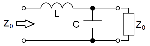
A loss-less coaxial cable has inductance and capacitance and, their associated formulas introduce $ϵ$ and $\mu$. But, to home-in on the velocity of propagation, the characteristic impedance must also be determined. We can avoid the complexity of the telegrapher's equations by looking at a short piece of loss-less cable in the frequency domain: -

When s, L and C are small, we can ignore the $s^{2}LC{Z}_0$ term, hence: -

And, $Z_0=\sqrt{{\displaystyle \frac{L}{C}}}$ (a well known formula).

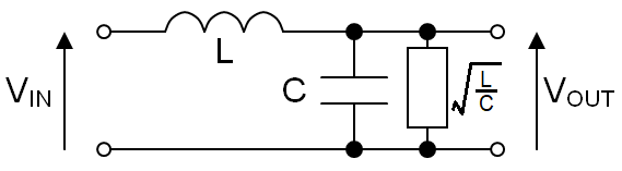
Having $Z_0$, we can analyse the circuit's transfer function. This allows us to find the output phase lag and, with a little more manipulation, the time delay for 1 metre of cable: -

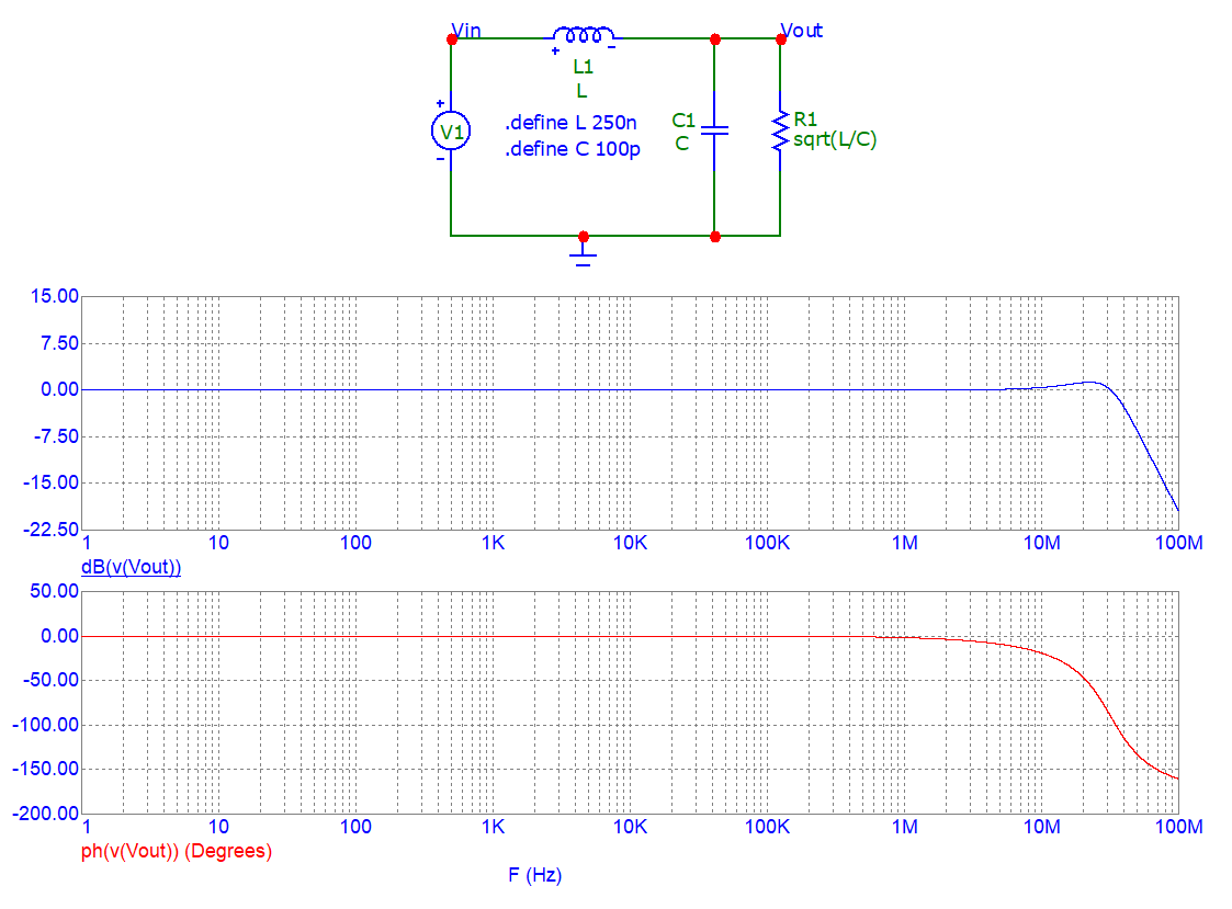
A general bode plot using lumped-values for L and C (per metre) is of interest: -

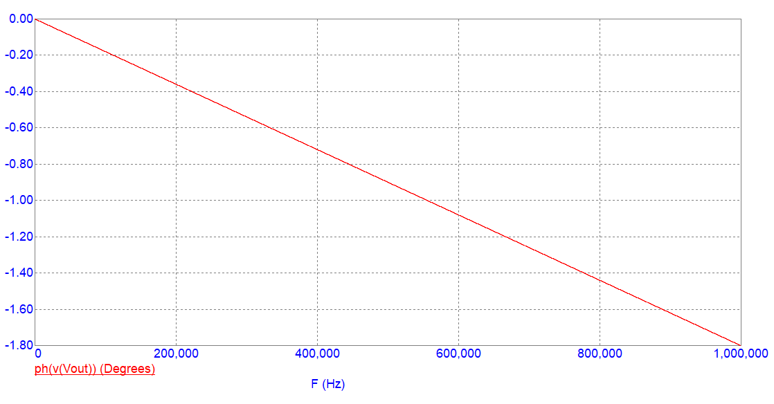
Here's a close-up of the phase response plotted linearly against frequency up to 1 MHz: -

• At 1 MHz, the output phase lag is 1.8°

• As a fraction of the period (1 μs) it's 0.005 hence, it's a time lag of 5 ns.

• At 100 kHz, the phase lag is 0.18° but, it's still a time lag of 5 ns

Because 1 metre lengths of capacitance and inductance are modelled, the equivalent velocity of propagation is 200 million metres per second (the inverse of the time lag).

A simulator is great as a demonstrator but, a phase angle formula is needed so that we know what the dependencies are. It's a simple 2nd order low pass filter and, if you went through the derivation (omitted to keep the answer shorter) you find this: -

Because we are making $\omega$ a lot smaller than ${\omega }_n$ we can simplify: -

• The arctan of a small number is the small number because $$\arctan (x)=x-\frac{x^3}{3}+\frac{x^5}{5}-...$$
• The denominator equals 1

But, we can also determine $\zeta$ for the circuit. Wikipedia RLC circuits shows it is this: -

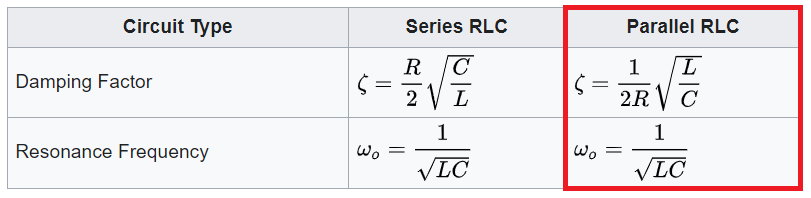
And, because we know that R is $Z_0$ $\left(\sqrt{\frac{L}{C}}\right)$, $\zeta$ must equal 0.5. The phase lag now becomes: -

_{Anyone studying telegrapher's equations will recognize this as the imaginary part of the propagation constant.$$$$}

Dividing the phase lag by $\omega$ gives us the time lag: -

And, the velocity of propagation is the reciprocal of the time lag (for a 1 metre length of cable): -

Nearly there!

Right at the start I mentioned coaxial cable and its inductance and capacitance per unit length. The formulas are: -

Taken from Inductance of a Coaxial Structure

Taken from Capacitance of a coaxial structure

If we multiply L and C we get $ϵ\cdot \mu$ hence,

posted over 1 year ago

CC BY-SA 4.0

1y ago

Andy aka‭

2329 reputation 19 76 269 284